LinearRegression: An implementation of ordinary least-squares linear regression

A implementation of Ordinary Least Squares simple and multiple linear regression.

from mlxtend.regressor import LinearRegression

Overview

Illustration of a simple linear regression model:

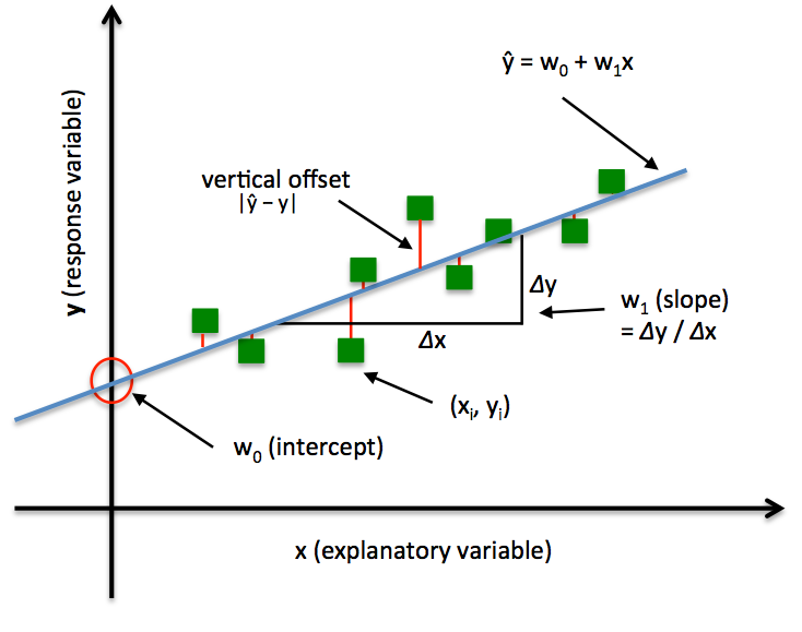
In Ordinary Least Squares (OLS) Linear Regression, our goal is to find the line (or hyperplane) that minimizes the vertical offsets. Or in other words, we define the best-fitting line as the line that minimizes the sum of squared errors (SSE) or mean squared error (MSE) between our target variable (y) and our predicted output over all samples $i$ in our dataset of size $n$ .

$SSE = \sum_i \big(\text{target}^{(i)} - \text{output}^{(i)}\big)^2$

$MSE = \frac{1}{n} \times SSE$

Now, LinearRegression implements a linear regression model for performing ordinary least squares regression using one of the following five approaches:

Normal Equations
QR Decomposition Method
SVD (Singular Value Decomposition) method
Gradient Descent
Stochastic Gradient Descent

Normal Equations (closed-form solution)

The closed-form solution should be preferred for "smaller" datasets where calculating (a "costly") matrix inverse is not a concern. For very large datasets, or datasets where the inverse of $[X^T X]$ may not exist (the matrix is non-invertible or singular, e.g., in case of perfect multicollinearity), the QR, SVD or gradient descent approaches are to be preferred.

The linear function (linear regression model) is defined as:

$y = w_0x_0 + w_1x_1 + ... + w_mx_m = \sum_{i=0}^{m} = \mathbf{w}^T\mathbf{x}$

where $y$ is the response variable, $\mathbf{x}$ is an $m$ -dimensional sample vector, and $\mathbf{w}$ is the weight vector (vector of coefficients). Note that $w_0$ represents the y-axis intercept of the model and therefore $x_0=1$ .

Using the closed-form solution (normal equation), we compute the weights of the model as follows:

$\mathbf{w} = (\mathbf{X}^T\mathbf{X})^{-1}\mathbf{X}^Ty$

Stable OLS via QR Factorization

The QR decomposition method offers a more numerically stable alternative to the closed-form, analytical solution based on the "normal equations," and it can be used to compute the inverse of large matrices more efficiently.

QR decomposition method decomposes given matrix into two matrices for which an inverse can be easily obtained. For instance, a given matrix $X \in \mathbb{R}^{n \times m}$ , the QR decomposition into two matrices is:

$\mathbf{X = QR},$

where

$Q \in \mathbb{R}^{n \times m}$ is an orthonormal matrix, such that $Q^\top Q = QQ^\top = I$ . The second matrix $R \in \mathbf{R}^{m \times m}$ is an upper triangular matrix.

The weight parameters of the ordinary least squares regression model can then be computed as follows [1]:

$\mathbf{w} = \mathbf{R}^{-1}\mathbf{Q}^\top y.$

Stable OLS via Singular Value Decomposition

Another alternative way for obtaining the OLS model weights in a numerically stable fashion is by Singular Value Decomposition (SVD), which is defined as:

$\mathbf{X}=\mathbf{U}\Sigma \mathbf{V}^\top,$

for a given matrix $\mathbf{X}$ .

Then, it can be shown that the pseudo-inverse of $X$ , $X^+$ , can be obtained as follows [1]:

$X^+ = \mathbf{U} \mathbf{\Sigma}^+ V^{\top}.$

Note that while $\Sigma$ is the diagonal matrix consisting of singular values of $\mathbf{X}$ , $\Sigma^{+}$ is the diagonal matrix consisting of the reciprocals of the singular values.

The model weights can then be computed as follows:

$\mathbf{w} = \mathbf{X}^+ \mathbf{y}.$

Please note that this OLS method is computationally most inefficient. However, it is a useful approach when the direct method (normal equations) or QR factorization cannot be applied or the normal equations (via $\mathbf{X}^T \mathbf{X}$ ) are ill-conditioned [3].

Gradient Descent (GD) and Stochastic Gradient Descent (SGD)

See Gradient Descent and Stochastic Gradient Descent and Deriving the Gradient Descent Rule for Linear Regression and Adaline for details.

Random shuffling is implemented as:

for one or more epochs
- randomly shuffle samples in the training set
  - for training sample i
    - compute gradients and perform weight updates

References

[1] Chapter 3, page 55, Linear Methods for Regression. Trevor Hastie; Robert Tibshirani; Jerome Friedman (2009). The Elements of Statistical Learning: Data Mining, Inference, and Prediction (2nd ed.). New York: Springer. (ISBN 978–0–387–84858–7)
[2] G. Strang, Linear Algebra and Its Applications, 2nd Ed., Orlando, FL, Academic Press, Inc., 1980, pp. 139-142.
[3] Douglas Wilhelm Harder. Numerical Analysis for Engineering. Section 4.8, ill-conditioned Matrices

Example 1 - Closed Form Solution

import numpy as np
import matplotlib.pyplot as plt
from mlxtend.regressor import LinearRegression

X = np.array([ 1.0, 2.1, 3.6, 4.2, 6])[:, np.newaxis]
y = np.array([ 1.0, 2.0, 3.0, 4.0, 5.0])

ne_lr = LinearRegression()
ne_lr.fit(X, y)

print('Intercept: %.2f' % ne_lr.b_)
print('Slope: %.2f' % ne_lr.w_[0])

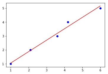
def lin_regplot(X, y, model):
    plt.scatter(X, y, c='blue')
    plt.plot(X, model.predict(X), color='red')    
    return

lin_regplot(X, y, ne_lr)
plt.show()

Intercept: 0.25
Slope: 0.81

png

Example 2 - QR decomposition method

import numpy as np
import matplotlib.pyplot as plt
from mlxtend.regressor import LinearRegression

X = np.array([ 1.0, 2.1, 3.6, 4.2, 6])[:, np.newaxis]
y = np.array([ 1.0, 2.0, 3.0, 4.0, 5.0])

qr_lr = LinearRegression(method='qr')
qr_lr.fit(X, y)

print('Intercept: %.2f' % qr_lr.b_)
print('Slope: %.2f' % qr_lr.w_[0])

def lin_regplot(X, y, model):
    plt.scatter(X, y, c='blue')
    plt.plot(X, model.predict(X), color='red')    
    return

lin_regplot(X, y, qr_lr)
plt.show()

Intercept: 0.25
Slope: 0.81

png

Example 3 - SVD method

import numpy as np
import matplotlib.pyplot as plt
from mlxtend.regressor import LinearRegression

X = np.array([ 1.0, 2.1, 3.6, 4.2, 6])[:, np.newaxis]
y = np.array([ 1.0, 2.0, 3.0, 4.0, 5.0])

svd_lr = LinearRegression(method='svd')
svd_lr.fit(X, y)

print('Intercept: %.2f' %svd_lr.b_)
print('Slope: %.2f' % svd_lr.w_[0])

def lin_regplot(X, y, model):
    plt.scatter(X, y, c='blue')
    plt.plot(X, model.predict(X), color='red')    
    return

lin_regplot(X, y, svd_lr)
plt.show()

Intercept: 0.25
Slope: 0.81

png

Example 4 - Gradient Descent

import numpy as np
import matplotlib.pyplot as plt
from mlxtend.regressor import LinearRegression

X = np.array([ 1.0, 2.1, 3.6, 4.2, 6])[:, np.newaxis]
y = np.array([ 1.0, 2.0, 3.0, 4.0, 5.0])

gd_lr = LinearRegression(method='sgd',
                         eta=0.005, 
                         epochs=100,
                         minibatches=1,
                         random_seed=123,
                         print_progress=3)
gd_lr.fit(X, y)

print('Intercept: %.2f' % gd_lr.b_)
print('Slope: %.2f' % gd_lr.w_)

def lin_regplot(X, y, model):
    plt.scatter(X, y, c='blue')
    plt.plot(X, model.predict(X), color='red')    
    return

lin_regplot(X, y, gd_lr)
plt.show()

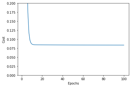
Iteration: 100/100 | Cost 0.08 | Elapsed: 0:00:00 | ETA: 0:00:00

Intercept: 0.22
Slope: 0.82

png

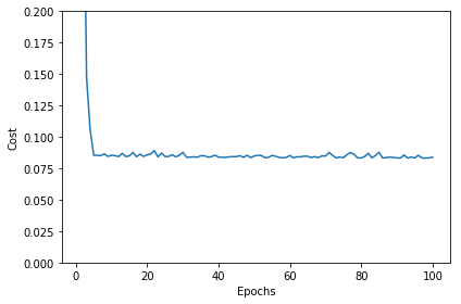
# Visualizing the cost to check for convergence and plotting the linear model:

plt.plot(range(1, gd_lr.epochs+1), gd_lr.cost_)
plt.xlabel('Epochs')
plt.ylabel('Cost')
plt.ylim([0, 0.2])
plt.tight_layout()
plt.show()

png

Example 5 - Stochastic Gradient Descent

import numpy as np
import matplotlib.pyplot as plt
from mlxtend.regressor import LinearRegression

X = np.array([ 1.0, 2.1, 3.6, 4.2, 6])[:, np.newaxis]
y = np.array([ 1.0, 2.0, 3.0, 4.0, 5.0])

sgd_lr = LinearRegression(method='sgd',
                          eta=0.01, 
                          epochs=100, 
                          random_seed=0, 
                          minibatches=len(y))
sgd_lr.fit(X, y)

print('Intercept: %.2f' % sgd_lr.w_)
print('Slope: %.2f' % sgd_lr.b_)

def lin_regplot(X, y, model):
    plt.scatter(X, y, c='blue')
    plt.plot(X, model.predict(X), color='red')    
    return

lin_regplot(X, y, sgd_lr)
plt.show()

Intercept: 0.82
Slope: 0.24

png

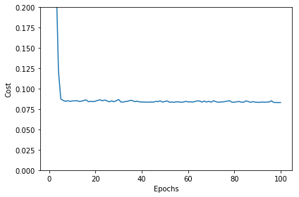
plt.plot(range(1, sgd_lr.epochs+1), sgd_lr.cost_)
plt.xlabel('Epochs')
plt.ylabel('Cost')
plt.ylim([0, 0.2])
plt.tight_layout()
plt.show()

png

Example 6 - Stochastic Gradient Descent with Minibatches

import numpy as np
import matplotlib.pyplot as plt
from mlxtend.regressor import LinearRegression

X = np.array([ 1.0, 2.1, 3.6, 4.2, 6])[:, np.newaxis]
y = np.array([ 1.0, 2.0, 3.0, 4.0, 5.0])

sgd_lr = LinearRegression(method='sgd',
                          eta=0.01, 
                          epochs=100, 
                          random_seed=0, 
                          minibatches=3)
sgd_lr.fit(X, y)

print('Intercept: %.2f' % sgd_lr.b_)
print('Slope: %.2f' % sgd_lr.w_)

def lin_regplot(X, y, model):
    plt.scatter(X, y, c='blue')
    plt.plot(X, model.predict(X), color='red')    
    return

lin_regplot(X, y, sgd_lr)
plt.show()

Intercept: 0.24
Slope: 0.82

png

plt.plot(range(1, sgd_lr.epochs+1), sgd_lr.cost_)
plt.xlabel('Epochs')
plt.ylabel('Cost')
plt.ylim([0, 0.2])
plt.tight_layout()
plt.show()

png

API

LinearRegression(method='direct', eta=0.01, epochs=50, minibatches=None, random_seed=None, print_progress=0)

Ordinary least squares linear regression.

Parameters

method : string (default: 'direct')

For gradient descent-based optimization, use sgd (see minibatch parameter for further options). Otherwise, if direct (default), the analytical method is used. For alternative, numerically more stable solutions, use either qr (QR decomopisition) or svd (Singular Value Decomposition).
eta : float (default: 0.01)

solver learning rate (between 0.0 and 1.0). Used with method = 'sgd'. (See methods parameter for details)
epochs : int (default: 50)

Passes over the training dataset. Prior to each epoch, the dataset is shuffled if minibatches > 1 to prevent cycles in stochastic gradient descent. Used with method = 'sgd'. (See methods parameter for details)
minibatches : int (default: None)

The number of minibatches for gradient-based optimization. If None: Direct method, QR, or SVD method (see method parameter for details) If 1: Gradient Descent learning If len(y): Stochastic Gradient Descent learning If 1 < minibatches < len(y): Minibatch learning
random_seed : int (default: None)

Set random state for shuffling and initializing the weights. Used in method = 'sgd'. (See methods parameter for details)
print_progress : int (default: 0)

Prints progress in fitting to stderr if method = 'sgd'. 0: No output 1: Epochs elapsed and cost 2: 1 plus time elapsed 3: 2 plus estimated time until completion

Attributes

w_ : 2d-array, shape={n_features, 1}

Model weights after fitting.
b_ : 1d-array, shape={1,}

Bias unit after fitting.
cost_ : list

Sum of squared errors after each epoch; ignored if solver='normal equation'

Examples

For usage examples, please see https://rasbt.github.io/mlxtend/user_guide/regressor/LinearRegression/

Methods

fit(X, y, init_params=True)

Learn model from training data.

Parameters

X : {array-like, sparse matrix}, shape = [n_samples, n_features]

Training vectors, where n_samples is the number of samples and n_features is the number of features.
y : array-like, shape = [n_samples]

Target values.
init_params : bool (default: True)

Re-initializes model parameters prior to fitting. Set False to continue training with weights from a previous model fitting.

Returns

self : object

get_params(deep=True)

Get parameters for this estimator.

Parameters

deep : boolean, optional

If True, will return the parameters for this estimator and contained subobjects that are estimators.

Returns

params : mapping of string to any

Parameter names mapped to their values.'

adapted from https://github.com/scikit-learn/scikit-learn/blob/master/sklearn/base.py Author: Gael Varoquaux gael.varoquaux@normalesup.org License: BSD 3 clause

predict(X)

Predict targets from X.

Parameters

X : {array-like, sparse matrix}, shape = [n_samples, n_features]

Training vectors, where n_samples is the number of samples and n_features is the number of features.

Returns

target_values : array-like, shape = [n_samples]

Predicted target values.

set_params(params)

Set the parameters of this estimator. The method works on simple estimators as well as on nested objects (such as pipelines). The latter have parameters of the form <component>__<parameter> so that it's possible to update each component of a nested object.

Returns

self

adapted from https://github.com/scikit-learn/scikit-learn/blob/master/sklearn/base.py Author: Gael Varoquaux gael.varoquaux@normalesup.org License: BSD 3 clause

ython

Keys	Action
`?`	Open this help
`n`	Next page
`p`	Previous page
`s`	Search