confusion_matrix: creating a confusion matrix for model evaluation

Functions for generating confusion matrices.

from mlxtend.evaluate import confusion_matrix
from mlxtend.plotting import plot_confusion_matrix

Overview

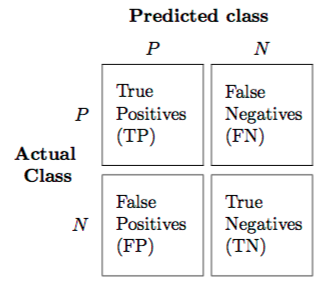
Confusion Matrix

The confusion matrix (or error matrix) is one way to summarize the performance of a classifier for binary classification tasks. This square matrix consists of columns and rows that list the number of instances as absolute or relative "actual class" vs. "predicted class" ratios.

Let $P$ be the label of class 1 and $N$ be the label of a second class or the label of all classes that are not class 1 in a multi-class setting.

References

• -

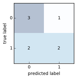
Example 1 - Binary classification

from mlxtend.evaluate import confusion_matrix

y_target =    [0, 0, 1, 0, 0, 1, 1, 1]
y_predicted = [1, 0, 1, 0, 0, 0, 0, 1]

cm = confusion_matrix(y_target=y_target, 
                      y_predicted=y_predicted)
cm

array([[3, 1],
       [2, 2]])

To visualize the confusion matrix using matplotlib, see the utility function mlxtend.plotting.plot_confusion_matrix:

import matplotlib.pyplot as plt
from mlxtend.plotting import plot_confusion_matrix

fig, ax = plot_confusion_matrix(conf_mat=cm)
plt.show()

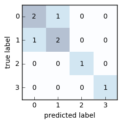
Example 2 - Multi-class classification

from mlxtend.evaluate import confusion_matrix

y_target =    [1, 1, 1, 0, 0, 2, 0, 3]
y_predicted = [1, 0, 1, 0, 0, 2, 1, 3]

cm = confusion_matrix(y_target=y_target, 
                      y_predicted=y_predicted, 
                      binary=False)
cm

array([[2, 1, 0, 0],
       [1, 2, 0, 0],
       [0, 0, 1, 0],
       [0, 0, 0, 1]])

To visualize the confusion matrix using matplotlib, see the utility function mlxtend.plotting.plot_confusion_matrix:

import matplotlib.pyplot as plt
from mlxtend.evaluate import confusion_matrix

fig, ax = plot_confusion_matrix(conf_mat=cm)
plt.show()

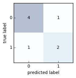
Example 3 - Multi-class to binary

By setting binary=True, all class labels that are not the positive class label are being summarized to class 0. The positive class label becomes class 1.

import matplotlib.pyplot as plt
from mlxtend.evaluate import confusion_matrix

y_target =    [1, 1, 1, 0, 0, 2, 0, 3]
y_predicted = [1, 0, 1, 0, 0, 2, 1, 3]

cm = confusion_matrix(y_target=y_target, 
                      y_predicted=y_predicted, 
                      binary=True, 
                      positive_label=1)
cm

array([[4, 1],
       [1, 2]])

To visualize the confusion matrix using matplotlib, see the utility function mlxtend.plotting.plot_confusion_matrix:

from mlxtend.plotting import plot_confusion_matrix

fig, ax = plot_confusion_matrix(conf_mat=cm)
plt.show()

API

confusion_matrix(y_target, y_predicted, binary=False, positive_label=1)

Compute a confusion matrix/contingency table.

Parameters

• y_target : array-like, shape=[n_samples]

  True class labels.

• y_predicted : array-like, shape=[n_samples]

  Predicted class labels.

• binary : bool (default: False)

  Maps a multi-class problem onto a binary confusion matrix, where the positive class is 1 and all other classes are 0.

• positive_label : int (default: 1)

  Class label of the positive class.

Returns

• mat : array-like, shape=[n_classes, n_classes]

Examples

For usage examples, please see https://rasbt.github.io/mlxtend/user_guide/evaluate/confusion_matrix/