plot_decision_regions: Visualize the decision regions of a classifier
A function for plotting decision regions of classifiers in 1 or 2 dimensions.
from mlxtend.plotting import plot_decision_regions
References
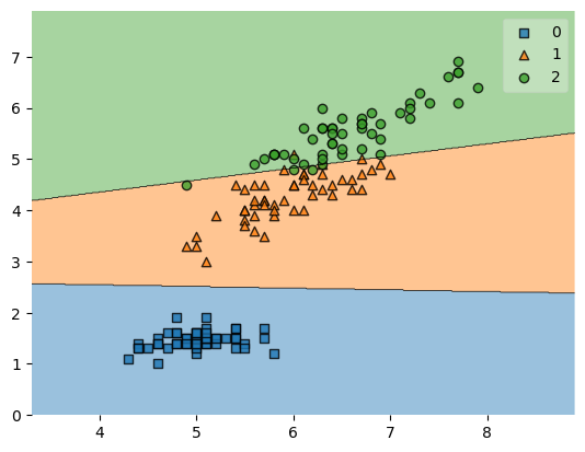
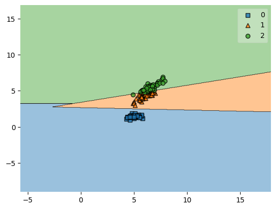
Example 1 - Decision regions in 2D
from mlxtend.plotting import plot_decision_regions
import matplotlib.pyplot as plt
from sklearn import datasets
from sklearn.svm import SVC

# Loading some example data
iris = datasets.load_iris()
X = iris.data[:, [0, 2]]
y = iris.target

# Training a classifier
svm = SVC(C=0.5, kernel='linear')
svm.fit(X, y)


# Plotting decision regions
plot_decision_regions(X, y, clf=svm, legend=2)

# Adding axes annotations
plt.xlabel('sepal length [cm]')
plt.ylabel('petal length [cm]')
plt.title('SVM on Iris')
plt.show()

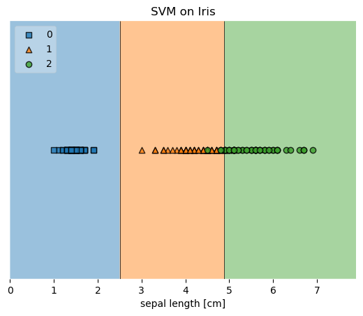
Example 2 - Decision regions in 1D
from mlxtend.plotting import plot_decision_regions
import matplotlib.pyplot as plt
from sklearn import datasets
from sklearn.svm import SVC

# Loading some example data
iris = datasets.load_iris()
X = iris.data[:, 2]
X = X[:, None]
y = iris.target

# Training a classifier
svm = SVC(C=0.5, kernel='linear')
svm.fit(X, y)

# Plotting decision regions
plot_decision_regions(X, y, clf=svm, legend=2)

# Adding axes annotations
plt.xlabel('sepal length [cm]')
plt.title('SVM on Iris')

plt.show()
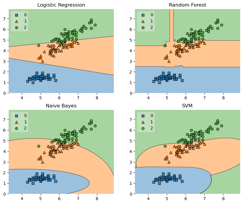
Example 3 - Decision Region Grids
from sklearn.linear_model import LogisticRegression
from sklearn.naive_bayes import GaussianNB
from sklearn.ensemble import RandomForestClassifier
from sklearn.svm import SVC
from sklearn import datasets
import numpy as np

# Initializing Classifiers
clf1 = LogisticRegression(random_state=1,
                          solver='newton-cg',
                          multi_class='multinomial')
clf2 = RandomForestClassifier(random_state=1, n_estimators=100)
clf3 = GaussianNB()
clf4 = SVC(gamma='auto')

# Loading some example data
iris = datasets.load_iris()
X = iris.data[:, [0,2]]
y = iris.target
import matplotlib.pyplot as plt
from mlxtend.plotting import plot_decision_regions
import matplotlib.gridspec as gridspec
import itertools
gs = gridspec.GridSpec(2, 2)

fig = plt.figure(figsize=(10,8))

labels = ['Logistic Regression', 'Random Forest', 'Naive Bayes', 'SVM']
for clf, lab, grd in zip([clf1, clf2, clf3, clf4],
                         labels,
                         itertools.product([0, 1], repeat=2)):

    clf.fit(X, y)
    ax = plt.subplot(gs[grd[0], grd[1]])
    fig = plot_decision_regions(X=X, y=y, clf=clf, legend=2)
    plt.title(lab)

plt.show()
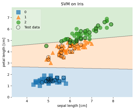
Example 4 - Highlighting Test Data Points
from mlxtend.plotting import plot_decision_regions
from mlxtend.preprocessing import shuffle_arrays_unison
import matplotlib.pyplot as plt
from sklearn import datasets
from sklearn.svm import SVC


# Loading some example data
iris = datasets.load_iris()
X, y = iris.data[:, [0,2]], iris.target
X, y = shuffle_arrays_unison(arrays=[X, y], random_seed=3)

X_train, y_train = X[:100], y[:100]
X_test, y_test = X[100:], y[100:]

# Training a classifier
svm = SVC(C=0.5, kernel='linear')
svm.fit(X_train, y_train)

# Plotting decision regions
plot_decision_regions(X, y, clf=svm, legend=2,
                      X_highlight=X_test)

# Adding axes annotations
plt.xlabel('sepal length [cm]')
plt.ylabel('petal length [cm]')
plt.title('SVM on Iris')
plt.show()
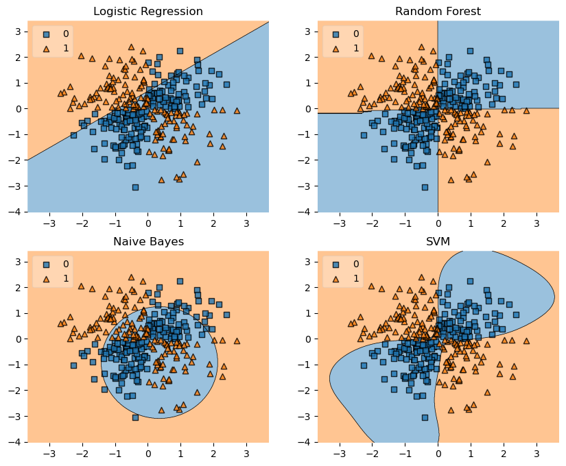
Example 5 - Evaluating Classifier Behavior on Non-Linear Problems
from sklearn.linear_model import LogisticRegression
from sklearn.naive_bayes import GaussianNB
from sklearn.ensemble import RandomForestClassifier
from sklearn.svm import SVC

# Initializing Classifiers
clf1 = LogisticRegression(random_state=1, solver='lbfgs')
clf2 = RandomForestClassifier(n_estimators=100,
                              random_state=1)
clf3 = GaussianNB()
clf4 = SVC(gamma='auto')
# Loading Plotting Utilities
import matplotlib.pyplot as plt
import matplotlib.gridspec as gridspec
import itertools
from mlxtend.plotting import plot_decision_regions
import numpy as np
XOR
xx, yy = np.meshgrid(np.linspace(-3, 3, 50),
                     np.linspace(-3, 3, 50))
rng = np.random.RandomState(0)
X = rng.randn(300, 2)
y = np.array(np.logical_xor(X[:, 0] > 0, X[:, 1] > 0),
             dtype=int)
gs = gridspec.GridSpec(2, 2)

fig = plt.figure(figsize=(10,8))

labels = ['Logistic Regression', 'Random Forest', 'Naive Bayes', 'SVM']
for clf, lab, grd in zip([clf1, clf2, clf3, clf4],
                         labels,
                         itertools.product([0, 1], repeat=2)):

    clf.fit(X, y)
    ax = plt.subplot(gs[grd[0], grd[1]])
    fig = plot_decision_regions(X=X, y=y, clf=clf, legend=2)
    plt.title(lab)

plt.show()
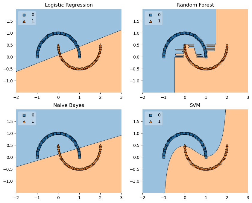
Half-Moons
from sklearn.datasets import make_moons
X, y = make_moons(n_samples=100, random_state=123)

gs = gridspec.GridSpec(2, 2)

fig = plt.figure(figsize=(10,8))

labels = ['Logistic Regression', 'Random Forest', 'Naive Bayes', 'SVM']
for clf, lab, grd in zip([clf1, clf2, clf3, clf4],
                         labels,
                         itertools.product([0, 1], repeat=2)):

    clf.fit(X, y)
    ax = plt.subplot(gs[grd[0], grd[1]])
    fig = plot_decision_regions(X=X, y=y, clf=clf, legend=2)
    plt.title(lab)

plt.show()
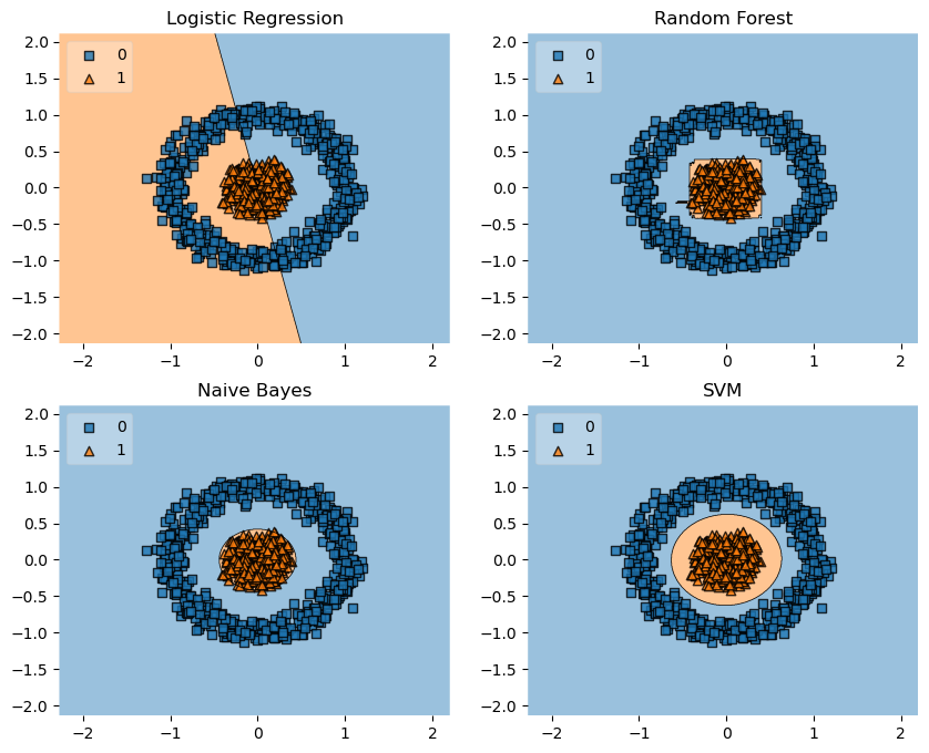
Concentric Circles
from sklearn.datasets import make_circles
X, y = make_circles(n_samples=1000, random_state=123, noise=0.1, factor=0.2)

gs = gridspec.GridSpec(2, 2)

fig = plt.figure(figsize=(10,8))

labels = ['Logistic Regression', 'Random Forest', 'Naive Bayes', 'SVM']
for clf, lab, grd in zip([clf1, clf2, clf3, clf4],
                         labels,
                         itertools.product([0, 1], repeat=2)):

    clf.fit(X, y)
    ax = plt.subplot(gs[grd[0], grd[1]])
    fig = plot_decision_regions(X=X, y=y, clf=clf, legend=2)
    plt.title(lab)

plt.show()
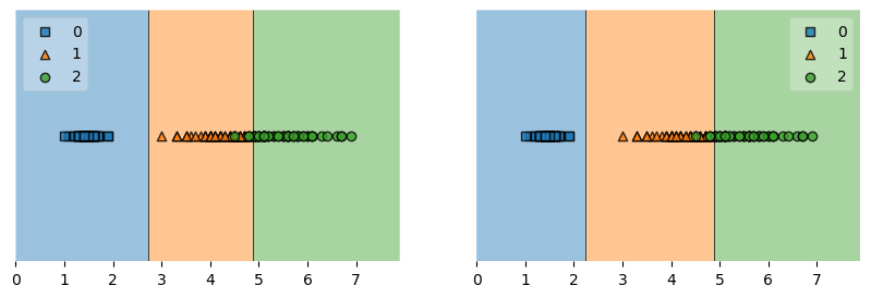
Example 6 - Working with existing axes objects using subplots
import matplotlib.pyplot as plt
from mlxtend.plotting import plot_decision_regions

from sklearn.linear_model import LogisticRegression
from sklearn.naive_bayes import GaussianNB
from sklearn import datasets
import numpy as np

# Loading some example data
iris = datasets.load_iris()
X = iris.data[:, 2]
X = X[:, None]
y = iris.target

# Initializing and fitting classifiers
clf1 = LogisticRegression(random_state=1,
                          solver='lbfgs',
                          multi_class='multinomial')
clf2 = GaussianNB()
clf1.fit(X, y)
clf2.fit(X, y)

fig, axes = plt.subplots(1, 2, figsize=(10, 3))

fig = plot_decision_regions(X=X, y=y, clf=clf1, ax=axes[0], legend=2)
fig = plot_decision_regions(X=X, y=y, clf=clf2, ax=axes[1], legend=1)

plt.show()
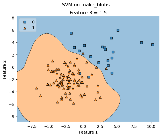
Example 7 - Decision regions with more than two training features
from mlxtend.plotting import plot_decision_regions
import matplotlib.pyplot as plt
from sklearn import datasets
from sklearn.svm import SVC

# Loading some example data
X, y = datasets.make_blobs(n_samples=600, n_features=3,
                           centers=[[2, 2, -2],[-2, -2, 2]],
                           cluster_std=[2, 2], random_state=2)

# Training a classifier
svm = SVC(gamma='auto')
svm.fit(X, y)

# Plotting decision regions
fig, ax = plt.subplots()
# Decision region for feature 3 = 1.5
value = 1.5
# Plot training sample with feature 3 = 1.5 +/- 0.75
width = 0.75
plot_decision_regions(X, y, clf=svm,
                      filler_feature_values={2: value},
                      filler_feature_ranges={2: width},
                      legend=2, ax=ax)
ax.set_xlabel('Feature 1')
ax.set_ylabel('Feature 2')
ax.set_title('Feature 3 = {}'.format(value))

# Adding axes annotations
fig.suptitle('SVM on make_blobs')
plt.show()
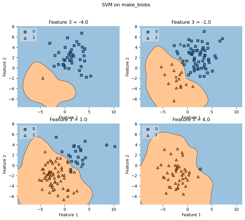
Example 8 - Grid of decision region slices
from mlxtend.plotting import plot_decision_regions
import matplotlib.pyplot as plt
from sklearn import datasets
from sklearn.svm import SVC

# Loading some example data
X, y = datasets.make_blobs(n_samples=500, n_features=3, centers=[[2, 2, -2],[-2, -2, 2]],
                           cluster_std=[2, 2], random_state=2)

# Training a classifier
svm = SVC(gamma='auto')
svm.fit(X, y)

# Plotting decision regions
fig, axarr = plt.subplots(2, 2, figsize=(10,8), sharex=True, sharey=True)
values = [-4.0, -1.0, 1.0, 4.0]
width = 0.75
for value, ax in zip(values, axarr.flat):
    plot_decision_regions(X, y, clf=svm,
                          filler_feature_values={2: value},
                          filler_feature_ranges={2: width},
                          legend=2, ax=ax)
    ax.set_xlabel('Feature 1')
    ax.set_ylabel('Feature 2')
    ax.set_title('Feature 3 = {}'.format(value))

# Adding axes annotations
fig.suptitle('SVM on make_blobs')
plt.show()
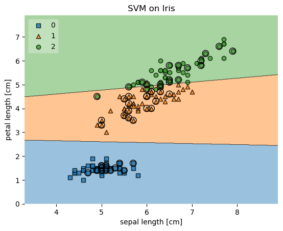
Example 9 - Customizing the plotting style
from mlxtend.plotting import plot_decision_regions
from mlxtend.preprocessing import shuffle_arrays_unison
import matplotlib.pyplot as plt
from sklearn import datasets
from sklearn.svm import SVC

# Loading some example data
iris = datasets.load_iris()
X = iris.data[:, [0, 2]]
y = iris.target
X, y = shuffle_arrays_unison(arrays=[X, y], random_seed=3)
X_train, y_train = X[:100], y[:100]
X_test, y_test = X[100:], y[100:]

# Training a classifier
svm = SVC(C=0.5, kernel='linear')
svm.fit(X_train, y_train)

# Specify keyword arguments to be passed to underlying plotting functions
scatter_kwargs = {'s': 120, 'edgecolor': None, 'alpha': 0.7}
contourf_kwargs = {'alpha': 0.2}
scatter_highlight_kwargs = {'s': 120, 'label': 'Test data', 'alpha': 0.7}
# Plotting decision regions
plot_decision_regions(X, y, clf=svm, legend=2,
                      X_highlight=X_test,
                      scatter_kwargs=scatter_kwargs,
                      contourf_kwargs=contourf_kwargs,
                      scatter_highlight_kwargs=scatter_highlight_kwargs)

# Adding axes annotations
plt.xlabel('sepal length [cm]')
plt.ylabel('petal length [cm]')
plt.title('SVM on Iris')
plt.show()
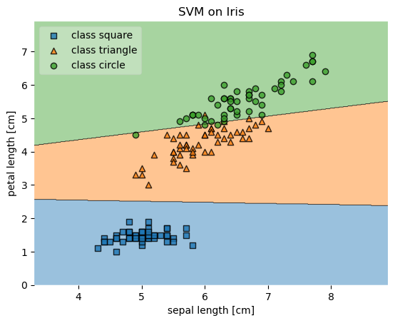
Example 10 - Providing your own legend labels
Custom legend labels can be provided by returning the axis object(s) from the plot_decision_region function and then getting the handles and labels of the legend. Custom handles (i.e., labels) can then be provided via ax.legend
ax = plot_decision_regions(X, y, clf=svm, legend=0)

handles, labels = ax.get_legend_handles_labels()
ax.legend(handles,
          ['class 0', 'class 1', 'class 2'],
           framealpha=0.3, scatterpoints=1)
An example is shown below.
from mlxtend.plotting import plot_decision_regions
import matplotlib.pyplot as plt
from sklearn import datasets
from sklearn.svm import SVC

# Loading some example data
iris = datasets.load_iris()
X = iris.data[:, [0, 2]]
y = iris.target

# Training a classifier
svm = SVC(C=0.5, kernel='linear')
svm.fit(X, y)


# Plotting decision regions
ax = plot_decision_regions(X, y, clf=svm, legend=0)

# Adding axes annotations
plt.xlabel('sepal length [cm]')
plt.ylabel('petal length [cm]')
plt.title('SVM on Iris')

handles, labels = ax.get_legend_handles_labels()
ax.legend(handles,
          ['class square', 'class triangle', 'class circle'],
           framealpha=0.3, scatterpoints=1)

plt.show()
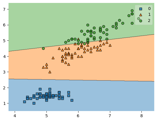
Example 11 - Plots with different zoom factors
from mlxtend.plotting import plot_decision_regions
import matplotlib.pyplot as plt
from sklearn import datasets
from sklearn.svm import SVC

# Loading some example data
iris = datasets.load_iris()
X = iris.data[:, [0, 2]]
y = iris.target

# Training a classifier
svm = SVC(C=0.5, kernel='linear')
svm.fit(X, y)
SVC(C=0.5, kernel='linear')In a Jupyter environment, please rerun this cell to show the HTML representation or trust the notebook.
On GitHub, the HTML representation is unable to render, please try loading this page with nbviewer.org.
SVC(C=0.5, kernel='linear')
Default Zoom Factor
plot_decision_regions(X, y, clf=svm, zoom_factor=1.)
plt.show()
Zooming out
plot_decision_regions(X, y, clf=svm, zoom_factor=0.1)
plt.show()
Zooming in
Note that while zooming in (by choosing a zoom_factor > 1.0) the plots are still created such that all data points are shown in the plot.
plot_decision_regions(X, y, clf=svm, zoom_factor=2.0)
plt.show()
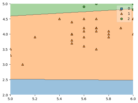
Cropping the axes
In order to zoom in further, which means that some training examples won't be shown, you can simply crop the axes as shown below:
plot_decision_regions(X, y, clf=svm, zoom_factor=2.0)
plt.xlim(5, 6)
plt.ylim(2, 5)
plt.show()
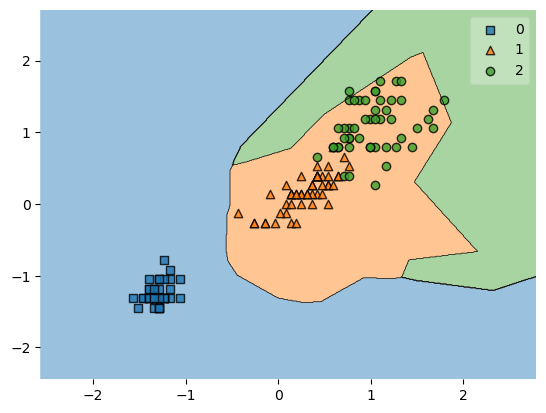
Example 12 - Using classifiers that expect onehot-encoded outputs (Keras)
Most objects for classification that mimick the scikit-learn estimator API should be compatible with the plot_decision_regions function. However, if the classification model (e.g., a typical Keras model) output onehot-encoded predictions, we have to use an additional trick. I.e., for onehot encoded outputs, we need to wrap the Keras model into a class that converts these onehot encoded variables into integers. Such a wrapper class can be as simple as the following:
class Onehot2Int(object):

    def __init__(self, model):
        self.model = model

    def predict(self, X):
        y_pred = self.model.predict(X)
        return np.argmax(y_pred, axis=1)
The example below illustrates how the Onehot2Int class can be used with a Keras model that outputs onehot encoded labels:
import keras
from keras.models import Sequential
from keras.layers import Dense
import matplotlib.pyplot as plt
import numpy as np
from mlxtend.data import iris_data
from mlxtend.preprocessing import standardize
from mlxtend.plotting import plot_decision_regions
from keras.utils import to_categorical

X, y = iris_data()
X = X[:, [2, 3]]

X = standardize(X)

# OneHot encoding
y_onehot = to_categorical(y)

# Create the model
np.random.seed(123)
model = Sequential()
model.add(Dense(8, input_shape=(2,), activation='relu', kernel_initializer='he_uniform'))
model.add(Dense(4, activation='relu', kernel_initializer='he_uniform'))
model.add(Dense(3, activation='softmax'))

# Configure the model and start training
model.compile(loss="categorical_crossentropy", optimizer=keras.optimizers.Adam(lr=0.005), metrics=['accuracy'])
history = model.fit(X, y_onehot, epochs=10, batch_size=5, verbose=1, validation_split=0.1)
Epoch 1/10
 1/27 [>.............................] - ETA: 3s - loss: 1.2769 - accuracy: 0.4000

/Users/sebastianraschka/miniforge3/envs/mlxtend/lib/python3.8/site-packages/keras/optimizers/optimizer_v2/adam.py:117: UserWarning: The `lr` argument is deprecated, use `learning_rate` instead.
  super().__init__(name, **kwargs)
2023-03-28 17:48:13.901264: W tensorflow/tsl/platform/profile_utils/cpu_utils.cc:128] Failed to get CPU frequency: 0 Hz


27/27 [==============================] - 0s 3ms/step - loss: 0.9526 - accuracy: 0.4222 - val_loss: 1.2656 - val_accuracy: 0.0000e+00
Epoch 2/10
27/27 [==============================] - 0s 834us/step - loss: 0.7062 - accuracy: 0.6741 - val_loss: 1.0939 - val_accuracy: 0.0000e+00
Epoch 3/10
27/27 [==============================] - 0s 808us/step - loss: 0.6461 - accuracy: 0.7111 - val_loss: 1.0705 - val_accuracy: 0.0667
Epoch 4/10
27/27 [==============================] - 0s 767us/step - loss: 0.6145 - accuracy: 0.7185 - val_loss: 1.0518 - val_accuracy: 0.0000e+00
Epoch 5/10
27/27 [==============================] - 0s 746us/step - loss: 0.5877 - accuracy: 0.7185 - val_loss: 1.0470 - val_accuracy: 0.0000e+00
Epoch 6/10
27/27 [==============================] - 0s 740us/step - loss: 0.5496 - accuracy: 0.7333 - val_loss: 1.0275 - val_accuracy: 0.0000e+00
Epoch 7/10
27/27 [==============================] - 0s 734us/step - loss: 0.4985 - accuracy: 0.7333 - val_loss: 1.0131 - val_accuracy: 0.0000e+00
Epoch 8/10
27/27 [==============================] - 0s 739us/step - loss: 0.4365 - accuracy: 0.7333 - val_loss: 0.9634 - val_accuracy: 0.0000e+00
Epoch 9/10
27/27 [==============================] - 0s 729us/step - loss: 0.3875 - accuracy: 0.7333 - val_loss: 0.9442 - val_accuracy: 0.0000e+00
Epoch 10/10
27/27 [==============================] - 0s 764us/step - loss: 0.3402 - accuracy: 0.7407 - val_loss: 0.8565 - val_accuracy: 0.0000e+00
# Wrap keras model
model_no_ohe = Onehot2Int(model)

# Plot decision boundary
plot_decision_regions(X, y, clf=model_no_ohe)
plt.show()
9600/9600 [==============================] - 3s 289us/step
API
plot_decision_regions(X, y, clf, feature_index=None, filler_feature_values=None, filler_feature_ranges=None, ax=None, X_highlight=None, zoom_factor=1.0, legend=1, hide_spines=True, markers='s^oxv<>', colors='#1f77b4,#ff7f0e,#3ca02c,#d62728,#9467bd,#8c564b,#e377c2,#7f7f7f,#bcbd22,#17becf', scatter_kwargs=None, contourf_kwargs=None, contour_kwargs=None, scatter_highlight_kwargs=None, n_jobs=None)
Plot decision regions of a classifier.
Please note that this functions assumes that class labels are
labeled consecutively, e.g,. 0, 1, 2, 3, 4, and 5. If you have class
labels with integer labels > 4, you may want to provide additional colors
and/or markers as `colors` and `markers` arguments.
See https://matplotlib.org/examples/color/named_colors.html for more
information.
Parameters
-
X: array-like, shape = [n_samples, n_features]Feature Matrix.
-
y: array-like, shape = [n_samples]True class labels.
-
clf: Classifier object.Must have a .predict method.
-
feature_index: array-like (default: (0,) for 1D, (0, 1) otherwise)Feature indices to use for plotting. The first index in
feature_indexwill be on the x-axis, the second index will be on the y-axis. -
filler_feature_values: dict (default: None)Only needed for number features > 2. Dictionary of feature index-value pairs for the features not being plotted.
-
filler_feature_ranges: dict (default: None)Only needed for number features > 2. Dictionary of feature index-value pairs for the features not being plotted. Will use the ranges provided to select training samples for plotting.
-
ax: matplotlib.axes.Axes (default: None)An existing matplotlib Axes. Creates one if ax=None.
-
X_highlight: array-like, shape = [n_samples, n_features] (default: None)An array with data points that are used to highlight samples in
X. -
zoom_factor: float (default: 1.0)Controls the scale of the x- and y-axis of the decision plot.
-
hide_spines: bool (default: True)Hide axis spines if True.
-
legend: int (default: 1)Integer to specify the legend location. No legend if legend is 0.
-
markers: str (default: 's^oxv<>')Scatterplot markers.
-
colors: str (default: 'red,blue,limegreen,gray,cyan')Comma separated list of colors.
-
scatter_kwargs: dict (default: None)Keyword arguments for underlying matplotlib scatter function.
-
contourf_kwargs: dict (default: None)Keyword arguments for underlying matplotlib contourf function.
-
contour_kwargs: dict (default: None)Keyword arguments for underlying matplotlib contour function (which draws the lines between decision regions).
-
scatter_highlight_kwargs: dict (default: None)Keyword arguments for underlying matplotlib scatter function.
-
n_jobs: int or None, optional (default=None)The number of CPUs to use to do the computation using Python's multiprocessing library.
Nonemeans 1.-1means using all processors. New in v0.22.0.
Returns
ax: matplotlib.axes.Axes object
Examples
For usage examples, please see https://rasbt.github.io/mlxtend/user_guide/plotting/plot_decision_regions/