Adaline: Adaptive Linear Neuron Classifier

An implementation of the ADAptive LInear NEuron, Adaline, for binary classification tasks.

from mlxtend.classifier import Adaline

Overview

An illustration of the ADAptive LInear NEuron (Adaline) -- a single-layer artificial linear neuron with a threshold unit:

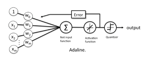
The Adaline classifier is closely related to the Ordinary Least Squares (OLS) Linear Regression algorithm; in OLS regression we find the line (or hyperplane) that minimizes the vertical offsets. Or in other words, we define the best-fitting line as the line that minimizes the sum of squared errors (SSE) or mean squared error (MSE) between our target variable (y) and our predicted output over all samples $i$ in our dataset of size $n$ .

$SSE = \sum_i (\text{target}^{(i)} - \text{output}^{(i)})^2$

$MSE = \frac{1}{n} \times SSE$

LinearRegression implements a linear regression model for performing ordinary least squares regression, and in Adaline, we add a threshold function $g(\cdot)$ to convert the continuous outcome to a categorical class label:

$$y = g({z}) = $\begin{cases} 1 & \text{if z $\ge$ 0}\\ -1 & \text{otherwise}. \end{cases}$ $$

An Adaline model can be trained by one of the following three approaches:

Normal Equations
Gradient Descent
Stochastic Gradient Descent

Normal Equations (closed-form solution)

The closed-form solution should be preferred for "smaller" datasets where calculating (a "costly") matrix inverse is not a concern. For very large datasets, or datasets where the inverse of $[X^T X]$ may not exist (the matrix is non-invertible or singular, e.g., in case of perfect multicollinearity), the gradient descent or stochastic gradient descent approaches are to be preferred.

The linear function (linear regression model) is defined as:

$z = w_0x_0 + w_1x_1 + ... + w_mx_m = \sum_{j=0}^{m} w_j x_j = \mathbf{w}^T\mathbf{x}$

where $y$ is the response variable, $\mathbf{x}$ is an $m$ -dimensional sample vector, and $\mathbf{w}$ is the weight vector (vector of coefficients). Note that $w_0$ represents the y-axis intercept of the model and therefore $x_0=1$ .

Using the closed-form solution (normal equation), we compute the weights of the model as follows:

$\mathbf{w} = (\mathbf{X}^T\mathbf{X})^{-1}\mathbf{X}^Ty$

Gradient Descent (GD) and Stochastic Gradient Descent (SGD)

In the current implementation, the Adaline model is learned via Gradient Descent or Stochastic Gradient Descent.

See Gradient Descent and Stochastic Gradient Descent and Deriving the Gradient Descent Rule for Linear Regression and Adaline for details.

Random shuffling is implemented as:

for one or more epochs
- randomly shuffle samples in the training set
  - for training sample i
    - compute gradients and perform weight updates

References

B. Widrow, M. E. Hoff, et al. Adaptive switching circuits. 1960.

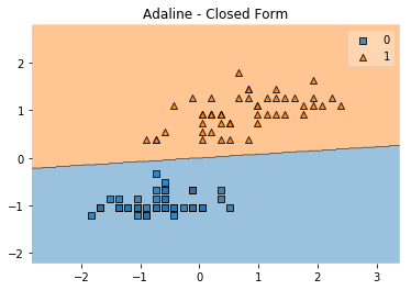
Example 1 - Closed Form Solution

from mlxtend.data import iris_data
from mlxtend.plotting import plot_decision_regions
from mlxtend.classifier import Adaline
import matplotlib.pyplot as plt

# Loading Data

X, y = iris_data()
X = X[:, [0, 3]] # sepal length and petal width
X = X[0:100] # class 0 and class 1
y = y[0:100] # class 0 and class 1

# standardize
X[:,0] = (X[:,0] - X[:,0].mean()) / X[:,0].std()
X[:,1] = (X[:,1] - X[:,1].mean()) / X[:,1].std()


ada = Adaline(epochs=30, 
              eta=0.01, 
              minibatches=None, 
              random_seed=1)
ada.fit(X, y)
plot_decision_regions(X, y, clf=ada)
plt.title('Adaline - Closed Form')

plt.show()

png

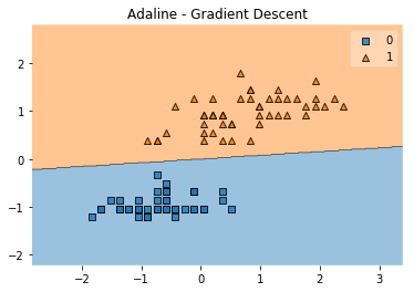
Example 2 - Gradient Descent

from mlxtend.data import iris_data
from mlxtend.plotting import plot_decision_regions
from mlxtend.classifier import Adaline
import matplotlib.pyplot as plt

# Loading Data

X, y = iris_data()
X = X[:, [0, 3]] # sepal length and petal width
X = X[0:100] # class 0 and class 1
y = y[0:100] # class 0 and class 1

# standardize
X[:,0] = (X[:,0] - X[:,0].mean()) / X[:,0].std()
X[:,1] = (X[:,1] - X[:,1].mean()) / X[:,1].std()


ada = Adaline(epochs=30, 
              eta=0.01, 
              minibatches=1, # for Gradient Descent Learning
              random_seed=1,
              print_progress=3)

ada.fit(X, y)
plot_decision_regions(X, y, clf=ada)
plt.title('Adaline - Gradient Descent')
plt.show()

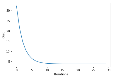
plt.plot(range(len(ada.cost_)), ada.cost_)
plt.xlabel('Iterations')
plt.ylabel('Cost')

Iteration: 30/30 | Cost 3.79 | Elapsed: 0:00:00 | ETA: 0:00:00

png

Text(0, 0.5, 'Cost')

png

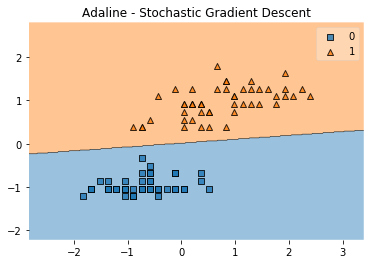
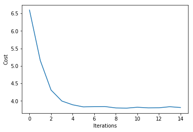
Example 3 - Stochastic Gradient Descent

from mlxtend.data import iris_data
from mlxtend.plotting import plot_decision_regions
from mlxtend.classifier import Adaline
import matplotlib.pyplot as plt

# Loading Data

X, y = iris_data()
X = X[:, [0, 3]] # sepal length and petal width
X = X[0:100] # class 0 and class 1
y = y[0:100] # class 0 and class 1

# standardize
X[:,0] = (X[:,0] - X[:,0].mean()) / X[:,0].std()
X[:,1] = (X[:,1] - X[:,1].mean()) / X[:,1].std()


ada = Adaline(epochs=15, 
              eta=0.02, 
              minibatches=len(y), # for SGD learning 
              random_seed=1,
              print_progress=3)

ada.fit(X, y)
plot_decision_regions(X, y, clf=ada)
plt.title('Adaline - Stochastic Gradient Descent')
plt.show()

plt.plot(range(len(ada.cost_)), ada.cost_)
plt.xlabel('Iterations')
plt.ylabel('Cost')
plt.show()

Iteration: 15/15 | Cost 3.81 | Elapsed: 0:00:00 | ETA: 0:00:00

png

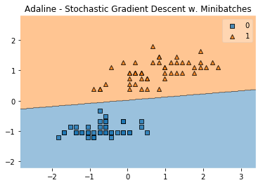
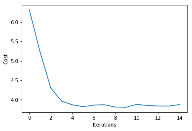
Example 4 - Stochastic Gradient Descent with Minibatches

from mlxtend.data import iris_data
from mlxtend.plotting import plot_decision_regions
from mlxtend.classifier import Adaline
import matplotlib.pyplot as plt

# Loading Data

X, y = iris_data()
X = X[:, [0, 3]] # sepal length and petal width
X = X[0:100] # class 0 and class 1
y = y[0:100] # class 0 and class 1

# standardize
X[:,0] = (X[:,0] - X[:,0].mean()) / X[:,0].std()
X[:,1] = (X[:,1] - X[:,1].mean()) / X[:,1].std()


ada = Adaline(epochs=15, 
              eta=0.02, 
              minibatches=5, # for SGD learning w. minibatch size 20
              random_seed=1,
              print_progress=3)

ada.fit(X, y)
plot_decision_regions(X, y, clf=ada)
plt.title('Adaline - Stochastic Gradient Descent w. Minibatches')
plt.show()

plt.plot(range(len(ada.cost_)), ada.cost_)
plt.xlabel('Iterations')
plt.ylabel('Cost')
plt.show()

Iteration: 15/15 | Cost 3.87 | Elapsed: 0:00:00 | ETA: 0:00:00

png

API

Adaline(eta=0.01, epochs=50, minibatches=None, random_seed=None, print_progress=0)

ADAptive LInear NEuron classifier.

Note that this implementation of Adaline expects binary class labels in {0, 1}.

Parameters

eta : float (default: 0.01)

solver rate (between 0.0 and 1.0)
epochs : int (default: 50)

Passes over the training dataset. Prior to each epoch, the dataset is shuffled if minibatches > 1 to prevent cycles in stochastic gradient descent.
minibatches : int (default: None)

The number of minibatches for gradient-based optimization. If None: Normal Equations (closed-form solution) If 1: Gradient Descent learning If len(y): Stochastic Gradient Descent (SGD) online learning If 1 < minibatches < len(y): SGD Minibatch learning
random_seed : int (default: None)

Set random state for shuffling and initializing the weights.
print_progress : int (default: 0)

Prints progress in fitting to stderr if not solver='normal equation' 0: No output 1: Epochs elapsed and cost 2: 1 plus time elapsed 3: 2 plus estimated time until completion

Attributes

w_ : 2d-array, shape={n_features, 1}

Model weights after fitting.
b_ : 1d-array, shape={1,}

Bias unit after fitting.
cost_ : list

Sum of squared errors after each epoch.

Examples

For usage examples, please see https://rasbt.github.io/mlxtend/user_guide/classifier/Adaline/

Methods

fit(X, y, init_params=True)

Learn model from training data.

Parameters

X : {array-like, sparse matrix}, shape = [n_samples, n_features]

Training vectors, where n_samples is the number of samples and n_features is the number of features.
y : array-like, shape = [n_samples]

Target values.
init_params : bool (default: True)

Re-initializes model parameters prior to fitting. Set False to continue training with weights from a previous model fitting.

Returns

self : object

get_params(deep=True)

Get parameters for this estimator.

Parameters

deep : boolean, optional

If True, will return the parameters for this estimator and contained subobjects that are estimators.

Returns

params : mapping of string to any

Parameter names mapped to their values.'

adapted from https://github.com/scikit-learn/scikit-learn/blob/master/sklearn/base.py Author: Gael Varoquaux gael.varoquaux@normalesup.org License: BSD 3 clause

predict(X)

Predict targets from X.

Parameters

X : {array-like, sparse matrix}, shape = [n_samples, n_features]

Training vectors, where n_samples is the number of samples and n_features is the number of features.

Returns

target_values : array-like, shape = [n_samples]

Predicted target values.

score(X, y)

Compute the prediction accuracy

Parameters

X : {array-like, sparse matrix}, shape = [n_samples, n_features]

Training vectors, where n_samples is the number of samples and n_features is the number of features.
y : array-like, shape = [n_samples]

Target values (true class labels).

Returns

acc : float

The prediction accuracy as a float between 0.0 and 1.0 (perfect score).

set_params(params)

Set the parameters of this estimator. The method works on simple estimators as well as on nested objects (such as pipelines). The latter have parameters of the form <component>__<parameter> so that it's possible to update each component of a nested object.

Returns

self

adapted from https://github.com/scikit-learn/scikit-learn/blob/master/sklearn/base.py Author: Gael Varoquaux gael.varoquaux@normalesup.org License: BSD 3 clause

Keys	Action
`?`	Open this help
`n`	Next page
`p`	Previous page
`s`	Search