ExhaustiveFeatureSelector: Optimal feature sets by considering all possible feature combinations

Implementation of an exhaustive feature selector for sampling and evaluating all possible feature combinations in a specified range.

from mlxtend.feature_selection import ExhaustiveFeatureSelector

Overview

This exhaustive feature selection algorithm is a wrapper approach for brute-force evaluation of feature subsets; the best subset is selected by optimizing a specified performance metric given an arbitrary regressor or classifier. For instance, if the classifier is a logistic regression and the dataset consists of 4 features, the alogorithm will evaluate all 15 feature combinations (if min_features=1 and max_features=4)

{0}
{1}
{2}
{3}
{0, 1}
{0, 2}
{0, 3}
{1, 2}
{1, 3}
{2, 3}
{0, 1, 2}
{0, 1, 3}
{0, 2, 3}
{1, 2, 3}
{0, 1, 2, 3}

and select the one that results in the best performance (e.g., classification accuracy) of the logistic regression classifier.

Example 1 - A simple Iris example

Initializing a simple classifier from scikit-learn:

from sklearn.neighbors import KNeighborsClassifier
from sklearn.datasets import load_iris
from mlxtend.feature_selection import ExhaustiveFeatureSelector as EFS

iris = load_iris()
X = iris.data
y = iris.target

knn = KNeighborsClassifier(n_neighbors=3)

efs1 = EFS(knn, 
           min_features=1,
           max_features=4,
           scoring='accuracy',
           print_progress=True,
           cv=5)

efs1 = efs1.fit(X, y)

print('Best accuracy score: %.2f' % efs1.best_score_)
print('Best subset (indices):', efs1.best_idx_)
print('Best subset (corresponding names):', efs1.best_feature_names_)

Features: 15/15

Best accuracy score: 0.97
Best subset (indices): (0, 2, 3)
Best subset (corresponding names): ('0', '2', '3')

Feature Names

When working with large datasets, the feature indices might be hard to interpret. In this case, we recommend using pandas DataFrames with distinct column names as input:

import pandas as pd

df_X = pd.DataFrame(X, columns=["Sepal length", "Sepal width", "Petal length", "Petal width"])
df_X.head()

	Sepal length	Sepal width	Petal length	Petal width
0	5.1	3.5	1.4	0.2
1	4.9	3.0	1.4	0.2
2	4.7	3.2	1.3	0.2
3	4.6	3.1	1.5	0.2
4	5.0	3.6	1.4	0.2

efs1 = efs1.fit(df_X, y)

print('Best accuracy score: %.2f' % efs1.best_score_)
print('Best subset (indices):', efs1.best_idx_)
print('Best subset (corresponding names):', efs1.best_feature_names_)

Features: 15/15

Best accuracy score: 0.97
Best subset (indices): (0, 2, 3)
Best subset (corresponding names): ('Sepal length', 'Petal length', 'Petal width')

Detailed Outputs

Via the subsets_ attribute, we can take a look at the selected feature indices at each step:

efs1.subsets_

{0: {'feature_idx': (0,),
  'cv_scores': array([0.53333333, 0.63333333, 0.7       , 0.8       , 0.56666667]),
  'avg_score': 0.6466666666666667,
  'feature_names': ('Sepal length',)},
 1: {'feature_idx': (1,),
  'cv_scores': array([0.43333333, 0.63333333, 0.53333333, 0.43333333, 0.5       ]),
  'avg_score': 0.5066666666666666,
  'feature_names': ('Sepal width',)},
 2: {'feature_idx': (2,),
  'cv_scores': array([0.93333333, 0.93333333, 0.9       , 0.93333333, 1.        ]),
  'avg_score': 0.9400000000000001,
  'feature_names': ('Petal length',)},
 3: {'feature_idx': (3,),
  'cv_scores': array([0.96666667, 0.96666667, 0.93333333, 0.93333333, 1.        ]),
  'avg_score': 0.96,
  'feature_names': ('Petal width',)},
 4: {'feature_idx': (0, 1),
  'cv_scores': array([0.66666667, 0.8       , 0.7       , 0.86666667, 0.66666667]),
  'avg_score': 0.74,
  'feature_names': ('Sepal length', 'Sepal width')},
 5: {'feature_idx': (0, 2),
  'cv_scores': array([0.96666667, 1.        , 0.86666667, 0.93333333, 0.96666667]),
  'avg_score': 0.9466666666666667,
  'feature_names': ('Sepal length', 'Petal length')},
 6: {'feature_idx': (0, 3),
  'cv_scores': array([0.96666667, 0.96666667, 0.9       , 0.93333333, 1.        ]),
  'avg_score': 0.9533333333333334,
  'feature_names': ('Sepal length', 'Petal width')},
 7: {'feature_idx': (1, 2),
  'cv_scores': array([0.93333333, 0.93333333, 0.9       , 0.93333333, 0.93333333]),
  'avg_score': 0.9266666666666667,
  'feature_names': ('Sepal width', 'Petal length')},
 8: {'feature_idx': (1, 3),
  'cv_scores': array([0.96666667, 0.96666667, 0.86666667, 0.93333333, 0.96666667]),
  'avg_score': 0.9400000000000001,
  'feature_names': ('Sepal width', 'Petal width')},
 9: {'feature_idx': (2, 3),
  'cv_scores': array([0.96666667, 0.96666667, 0.9       , 0.93333333, 1.        ]),
  'avg_score': 0.9533333333333334,
  'feature_names': ('Petal length', 'Petal width')},
 10: {'feature_idx': (0, 1, 2),
  'cv_scores': array([0.96666667, 0.96666667, 0.86666667, 0.93333333, 0.96666667]),
  'avg_score': 0.9400000000000001,
  'feature_names': ('Sepal length', 'Sepal width', 'Petal length')},
 11: {'feature_idx': (0, 1, 3),
  'cv_scores': array([0.93333333, 0.96666667, 0.9       , 0.93333333, 1.        ]),
  'avg_score': 0.9466666666666667,
  'feature_names': ('Sepal length', 'Sepal width', 'Petal width')},
 12: {'feature_idx': (0, 2, 3),
  'cv_scores': array([0.96666667, 0.96666667, 0.96666667, 0.96666667, 1.        ]),
  'avg_score': 0.9733333333333334,
  'feature_names': ('Sepal length', 'Petal length', 'Petal width')},
 13: {'feature_idx': (1, 2, 3),
  'cv_scores': array([0.96666667, 0.96666667, 0.93333333, 0.93333333, 1.        ]),
  'avg_score': 0.96,
  'feature_names': ('Sepal width', 'Petal length', 'Petal width')},
 14: {'feature_idx': (0, 1, 2, 3),
  'cv_scores': array([0.96666667, 0.96666667, 0.93333333, 0.96666667, 1.        ]),
  'avg_score': 0.9666666666666668,
  'feature_names': ('Sepal length',
   'Sepal width',
   'Petal length',
   'Petal width')}}

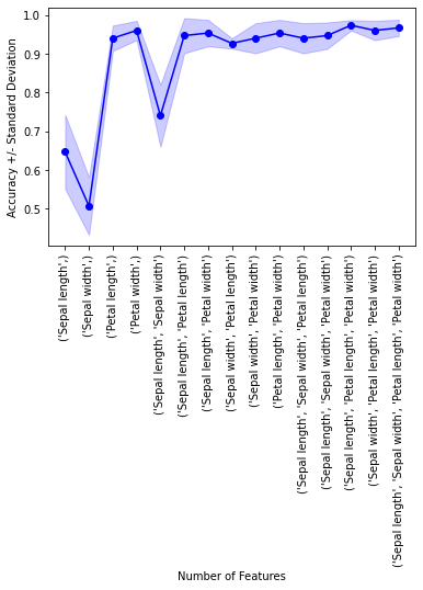
Example 2 - Visualizing the feature selection results

For our convenience, we can visualize the output from the feature selection in a pandas DataFrame format using the get_metric_dict method of the ExhaustiveFeatureSelector object. The columns std_dev and std_err represent the standard deviation and standard errors of the cross-validation scores, respectively.

Below, we see the DataFrame of the Sequential Forward Selector from Example 2:

import pandas as pd

iris = load_iris()
X = iris.data
y = iris.target

knn = KNeighborsClassifier(n_neighbors=3)

efs1 = EFS(knn, 
           min_features=1,
           max_features=4,
           scoring='accuracy',
           print_progress=True,
           cv=5)

feature_names = ('sepal length', 'sepal width',
                 'petal length', 'petal width')

df_X = pd.DataFrame(
    X, columns=["Sepal length", "Sepal width", "Petal length", "Petal width"])
efs1 = efs1.fit(df_X, y)

df = pd.DataFrame.from_dict(efs1.get_metric_dict()).T
df.sort_values('avg_score', inplace=True, ascending=False)
df

Features: 15/15

	feature_idx	cv_scores	avg_score	feature_names	ci_bound	std_dev	std_err
12	(0, 2, 3)	[0.9666666666666667, 0.9666666666666667, 0.966...	0.973333	(Sepal length, Petal length, Petal width)	0.017137	0.013333	0.006667
14	(0, 1, 2, 3)	[0.9666666666666667, 0.9666666666666667, 0.933...	0.966667	(Sepal length, Sepal width, Petal length, Peta...	0.027096	0.021082	0.010541
3	(3,)	[0.9666666666666667, 0.9666666666666667, 0.933...	0.96	(Petal width,)	0.032061	0.024944	0.012472
13	(1, 2, 3)	[0.9666666666666667, 0.9666666666666667, 0.933...	0.96	(Sepal width, Petal length, Petal width)	0.032061	0.024944	0.012472
6	(0, 3)	[0.9666666666666667, 0.9666666666666667, 0.9, ...	0.953333	(Sepal length, Petal width)	0.043691	0.033993	0.016997
9	(2, 3)	[0.9666666666666667, 0.9666666666666667, 0.9, ...	0.953333	(Petal length, Petal width)	0.043691	0.033993	0.016997
5	(0, 2)	[0.9666666666666667, 1.0, 0.8666666666666667, ...	0.946667	(Sepal length, Petal length)	0.058115	0.045216	0.022608
11	(0, 1, 3)	[0.9333333333333333, 0.9666666666666667, 0.9, ...	0.946667	(Sepal length, Sepal width, Petal width)	0.043691	0.033993	0.016997
2	(2,)	[0.9333333333333333, 0.9333333333333333, 0.9, ...	0.94	(Petal length,)	0.041977	0.03266	0.01633
8	(1, 3)	[0.9666666666666667, 0.9666666666666667, 0.866...	0.94	(Sepal width, Petal width)	0.049963	0.038873	0.019437
10	(0, 1, 2)	[0.9666666666666667, 0.9666666666666667, 0.866...	0.94	(Sepal length, Sepal width, Petal length)	0.049963	0.038873	0.019437
7	(1, 2)	[0.9333333333333333, 0.9333333333333333, 0.9, ...	0.926667	(Sepal width, Petal length)	0.017137	0.013333	0.006667
4	(0, 1)	[0.6666666666666666, 0.8, 0.7, 0.8666666666666...	0.74	(Sepal length, Sepal width)	0.102823	0.08	0.04
0	(0,)	[0.5333333333333333, 0.6333333333333333, 0.7, ...	0.646667	(Sepal length,)	0.122983	0.095685	0.047842
1	(1,)	[0.43333333333333335, 0.6333333333333333, 0.53...	0.506667	(Sepal width,)	0.095416	0.074237	0.037118

import matplotlib.pyplot as plt

metric_dict = efs1.get_metric_dict()

fig = plt.figure()
k_feat = sorted(metric_dict.keys())
avg = [metric_dict[k]['avg_score'] for k in k_feat]

upper, lower = [], []
for k in k_feat:
    upper.append(metric_dict[k]['avg_score'] +
                 metric_dict[k]['std_dev'])
    lower.append(metric_dict[k]['avg_score'] -
                 metric_dict[k]['std_dev'])

plt.fill_between(k_feat,
                 upper,
                 lower,
                 alpha=0.2,
                 color='blue',
                 lw=1)

plt.plot(k_feat, avg, color='blue', marker='o')
plt.ylabel('Accuracy +/- Standard Deviation')
plt.xlabel('Number of Features')
feature_min = len(metric_dict[k_feat[0]]['feature_idx'])
feature_max = len(metric_dict[k_feat[-1]]['feature_idx'])
plt.xticks(k_feat, 
           [str(metric_dict[k]['feature_names']) for k in k_feat], 
           rotation=90)
plt.show()

png

Example 3 - Exhaustive feature selection for regression analysis

Similar to the classification examples above, the SequentialFeatureSelector also supports scikit-learn's estimators for regression.

from sklearn.linear_model import LinearRegression
from sklearn.datasets import load_boston

boston = load_boston()
X, y = boston.data, boston.target

lr = LinearRegression()

efs = EFS(lr, 
          min_features=10,
          max_features=12,
          scoring='neg_mean_squared_error',
          cv=10)

efs.fit(X, y)

print('Best MSE score: %.2f' % efs.best_score_ * (-1))
print('Best subset:', efs.best_idx_)

/Users/sebastianraschka/miniforge3/lib/python3.9/site-packages/sklearn/utils/deprecation.py:87: FutureWarning: Function load_boston is deprecated; `load_boston` is deprecated in 1.0 and will be removed in 1.2.

    The Boston housing prices dataset has an ethical problem. You can refer to
    the documentation of this function for further details.

    The scikit-learn maintainers therefore strongly discourage the use of this
    dataset unless the purpose of the code is to study and educate about
    ethical issues in data science and machine learning.

    In this special case, you can fetch the dataset from the original
    source::

        import pandas as pd
        import numpy as np


        data_url = "http://lib.stat.cmu.edu/datasets/boston"
        raw_df = pd.read_csv(data_url, sep="\s+", skiprows=22, header=None)
        data = np.hstack([raw_df.values[::2, :], raw_df.values[1::2, :2]])
        target = raw_df.values[1::2, 2]

    Alternative datasets include the California housing dataset (i.e.
    :func:`~sklearn.datasets.fetch_california_housing`) and the Ames housing
    dataset. You can load the datasets as follows::

        from sklearn.datasets import fetch_california_housing
        housing = fetch_california_housing()

    for the California housing dataset and::

        from sklearn.datasets import fetch_openml
        housing = fetch_openml(name="house_prices", as_frame=True)

    for the Ames housing dataset.

  warnings.warn(msg, category=FutureWarning)
Features: 377/377


Best subset: (0, 1, 4, 6, 7, 8, 9, 10, 11, 12)

Example 4 - Regression and adjusted R2

As shown in Example 3, the exhaustive feature selector can be used for selecting features via a regression model. In regression analysis, there exists the common phenomenon that the $R^2$ score can become spuriously inflated the more features we choose. Hence, and this is especially true for feature selection, it is useful to make model comparisons based on the adjusted $R^2$ value rather than the regular $R^2$ . The adjusted $R^2$ , $\bar{R}^{2}$ , accounts for the number of features and examples as follows:

$\bar{R}^{2}=1-\left(1-R^{2}\right) \frac{n-1}{n-p-1},$

where $n$ is the number of examples and $p$ is the number of features.

One of the advantages of scikit-learn's API is that it's consistent, intuitive, and simple to use. However, one downside of this API design is that it can be a bit restrictive for certain scenarios. For instance, scikit-learn scoring function only take two inputs, the predicted and the true target values. Hence, we cannot use scikit-learn's scoring API to compute the adjusted $R^2$ , which also requires the number of features.

However, as a workaround, we can compute the $R^2$ for the different feature subsets and then do a posthoc computation to obtain the adjusted $R^2$ .

Step 1: Compute $R^2$ :

from sklearn.linear_model import LinearRegression
from sklearn.datasets import load_boston

boston = load_boston()
X, y = boston.data, boston.target

lr = LinearRegression()

efs = EFS(lr, 
          min_features=10,
          max_features=12,
          scoring='r2',
          cv=10)

efs.fit(X, y)

print('Best R2 score: %.2f' % efs.best_score_ * (-1))
print('Best subset:', efs.best_idx_)

/Users/sebastianraschka/miniforge3/lib/python3.9/site-packages/sklearn/utils/deprecation.py:87: FutureWarning: Function load_boston is deprecated; `load_boston` is deprecated in 1.0 and will be removed in 1.2.

    The Boston housing prices dataset has an ethical problem. You can refer to
    the documentation of this function for further details.

    The scikit-learn maintainers therefore strongly discourage the use of this
    dataset unless the purpose of the code is to study and educate about
    ethical issues in data science and machine learning.

    In this special case, you can fetch the dataset from the original
    source::

        import pandas as pd
        import numpy as np


        data_url = "http://lib.stat.cmu.edu/datasets/boston"
        raw_df = pd.read_csv(data_url, sep="\s+", skiprows=22, header=None)
        data = np.hstack([raw_df.values[::2, :], raw_df.values[1::2, :2]])
        target = raw_df.values[1::2, 2]

    Alternative datasets include the California housing dataset (i.e.
    :func:`~sklearn.datasets.fetch_california_housing`) and the Ames housing
    dataset. You can load the datasets as follows::

        from sklearn.datasets import fetch_california_housing
        housing = fetch_california_housing()

    for the California housing dataset and::

        from sklearn.datasets import fetch_openml
        housing = fetch_openml(name="house_prices", as_frame=True)

    for the Ames housing dataset.

  warnings.warn(msg, category=FutureWarning)
Features: 377/377


Best subset: (1, 3, 5, 6, 7, 8, 9, 10, 11, 12)

Step 2: Compute adjusted $R^2$ :

def adjust_r2(r2, num_examples, num_features):
    coef = (num_examples - 1) / (num_examples - num_features - 1) 
    return 1 - (1 - r2) * coef

for i in efs.subsets_:
    efs.subsets_[i]['adjusted_avg_score'] = (
        adjust_r2(r2=efs.subsets_[i]['avg_score'],
                  num_examples=X.shape[0]/10,
                  num_features=len(efs.subsets_[i]['feature_idx']))
    )

Step 3: Select best subset based on adjusted $R^2$ :

score = -99e10

for i in efs.subsets_:
    score = efs.subsets_[i]['adjusted_avg_score']
    if ( efs.subsets_[i]['adjusted_avg_score'] == score and
        len(efs.subsets_[i]['feature_idx']) < len(efs.best_idx_) )\
      or efs.subsets_[i]['adjusted_avg_score'] > score:
        efs.best_idx_ = efs.subsets_[i]['feature_idx']

print('Best adjusted R2 score: %.2f' % efs.best_score_ * (-1))
print('Best subset:', efs.best_idx_)

Best subset: (1, 3, 5, 6, 7, 8, 9, 10, 11, 12)

Example 5 - Using the selected feature subset For making new predictions

# Initialize the dataset

from sklearn.neighbors import KNeighborsClassifier
from sklearn.datasets import load_iris
from sklearn.model_selection import train_test_split

iris = load_iris()
X, y = iris.data, iris.target
X_train, X_test, y_train, y_test = train_test_split(
         X, y, test_size=0.33, random_state=1)

knn = KNeighborsClassifier(n_neighbors=3)

# Select the "best" three features via
# 5-fold cross-validation on the training set.

from mlxtend.feature_selection import ExhaustiveFeatureSelector as EFS

efs1 = EFS(knn, 
           min_features=1,
           max_features=4,
           scoring='accuracy',
           cv=5)
efs1 = efs1.fit(X_train, y_train)

Features: 15/15

print('Selected features:', efs1.best_idx_)

Selected features: (2, 3)

# Generate the new subsets based on the selected features
# Note that the transform call is equivalent to
# X_train[:, efs1.k_feature_idx_]

X_train_efs = efs1.transform(X_train)
X_test_efs = efs1.transform(X_test)

# Fit the estimator using the new feature subset
# and make a prediction on the test data
knn.fit(X_train_efs, y_train)
y_pred = knn.predict(X_test_efs)

# Compute the accuracy of the prediction
acc = float((y_test == y_pred).sum()) / y_pred.shape[0]
print('Test set accuracy: %.2f %%' % (acc*100))

Test set accuracy: 96.00 %

Example 6 - Exhaustive feature selection and GridSearch

# Initialize the dataset

from sklearn.datasets import load_iris
from sklearn.model_selection import train_test_split

iris = load_iris()
X, y = iris.data, iris.target
X_train, X_test, y_train, y_test = train_test_split(
         X, y, test_size=0.33, random_state=1)

Use scikit-learn's GridSearch to tune the hyperparameters of the LogisticRegression estimator inside the ExhaustiveFeatureSelector and use it for prediction in the pipeline. Note that the clone_estimator attribute needs to be set to False.

from sklearn.model_selection import GridSearchCV
from sklearn.pipeline import make_pipeline
from sklearn.linear_model import LogisticRegression
from mlxtend.feature_selection import ExhaustiveFeatureSelector as EFS

lr = LogisticRegression(multi_class='multinomial', 
                        solver='newton-cg', 
                        random_state=123)

efs1 = EFS(estimator=lr, 
           min_features=2,
           max_features=3,
           scoring='accuracy',
           print_progress=False,
           clone_estimator=False,
           cv=5,
           n_jobs=1)

pipe = make_pipeline(efs1, lr)

param_grid = {'exhaustivefeatureselector__estimator__C': [0.1, 1.0, 10.0]}

gs = GridSearchCV(estimator=pipe, 
                  param_grid=param_grid, 
                  scoring='accuracy', 
                  n_jobs=1, 
                  cv=2, 
                  verbose=1, 
                  refit=False)

# run gridearch
gs = gs.fit(X_train, y_train)

Fitting 2 folds for each of 3 candidates, totalling 6 fits

... and the "best" parameters determined by GridSearch are ...

print("Best parameters via GridSearch", gs.best_params_)

Best parameters via GridSearch {'exhaustivefeatureselector__estimator__C': 0.1}

Obtaining the best k feature indices after GridSearch

If we are interested in the best k best feature indices via SequentialFeatureSelection.best_idx_, we have to initialize a GridSearchCV object with refit=True. Now, the grid search object will take the complete training dataset and the best parameters, which it found via cross-validation, to train the estimator pipeline.

gs = GridSearchCV(estimator=pipe, 
                  param_grid=param_grid, 
                  scoring='accuracy', 
                  n_jobs=1, 
                  cv=2, 
                  verbose=1, 
                  refit=True)

After running the grid search, we can access the individual pipeline objects of the best_estimator_ via the steps attribute.

gs = gs.fit(X_train, y_train)
gs.best_estimator_.steps

Fitting 2 folds for each of 3 candidates, totalling 6 fits





[('exhaustivefeatureselector',
  ExhaustiveFeatureSelector(clone_estimator=False,
                            estimator=LogisticRegression(C=0.1,
                                                         multi_class='multinomial',
                                                         random_state=123,
                                                         solver='newton-cg'),
                            feature_groups=[[0], [1], [2], [3]], max_features=3,
                            min_features=2, print_progress=False)),
 ('logisticregression',
  LogisticRegression(multi_class='multinomial', random_state=123,
                     solver='newton-cg'))]

Via sub-indexing, we can then obtain the best-selected feature subset:

print('Best features:', gs.best_estimator_.steps[0][1].best_idx_)

Best features: (2, 3)

During cross-validation, this feature combination had a CV accuracy of:

print('Best score:', gs.best_score_)

Best score: 0.96

gs.best_params_

{'exhaustivefeatureselector__estimator__C': 0.1}

Alternatively, if we can set the "best grid search parameters" in our pipeline manually if we ran GridSearchCV with refit=False. It should yield the same results:

pipe.set_params(**gs.best_params_).fit(X_train, y_train)
print('Best features:', pipe.steps[0][1].best_idx_)

Best features: (2, 3)

Example 7 - Exhaustive Feature Selection with LOOCV

The ExhaustiveFeatureSelector is not restricted to k-fold cross-validation. You can use any type of cross-validation method that supports the general scikit-learn cross-validation API.

The following example illustrates the use of scikit-learn's LeaveOneOut cross-validation method in combination with the exhaustive feature selector.

from sklearn.neighbors import KNeighborsClassifier
from sklearn.datasets import load_iris
from mlxtend.feature_selection import ExhaustiveFeatureSelector as EFS
from sklearn.model_selection import LeaveOneOut


iris = load_iris()
X = iris.data
y = iris.target

knn = KNeighborsClassifier(n_neighbors=3)

efs1 = EFS(knn, 
           min_features=1,
           max_features=4,
           scoring='accuracy',
           print_progress=True,
           cv=LeaveOneOut()) ### Use cross-validation generator here

efs1 = efs1.fit(X, y)

print('Best accuracy score: %.2f' % efs1.best_score_)
print('Best subset (indices):', efs1.best_idx_)
print('Best subset (corresponding names):', efs1.best_feature_names_)

Features: 15/15

Best accuracy score: 0.96
Best subset (indices): (3,)
Best subset (corresponding names): ('3',)

Example 8 - Interrupting Long Runs for Intermediate Results

If your run is taking too long, it is possible to trigger a KeyboardInterrupt (e.g., ctrl+c on a Mac, or interrupting the cell in a Jupyter notebook) to obtain temporary results.

Toy dataset

from sklearn.datasets import make_classification
from sklearn.model_selection import train_test_split


X, y = make_classification(
    n_samples=200000,
    n_features=6,
    n_informative=2,
    n_redundant=1,
    n_repeated=1,
    n_clusters_per_class=2,
    flip_y=0.05,
    class_sep=0.5,
    random_state=123,
)

X_train, X_test, y_train, y_test = train_test_split(
    X, y, test_size=0.2, random_state=123
)

Long run with interruption

from mlxtend.feature_selection import ExhaustiveFeatureSelector as EFS
from sklearn.linear_model import LogisticRegression

model = LogisticRegression(max_iter=10000)

efs1 = EFS(model, 
           min_features=1, 
           max_features=4,
           print_progress=True,
           scoring='accuracy')

efs1 = efs1.fit(X_train, y_train)

Features: 56/56

Finalizing the fit

Note that the feature selection run hasn't finished, so certain attributes may not be available. In order to use the EFS instance, it is recommended to call finalize_fit, which will make EFS estimator appear as "fitted" process the temporary results:

efs1.finalize_fit()

print('Best accuracy score: %.2f' % efs1.best_score_)
print('Best subset (indices):', efs1.best_idx_)

Best accuracy score: 0.73
Best subset (indices): (1, 2)

Example 9 - Working with Feature Groups

Since mlxtend v0.21.0, it is possible to specify feature groups. Feature groups allow you to group certain features together, such that they are always selected as a group. This can be very useful in contexts similar to one-hot encoding -- if you want to treat the one-hot encoded feature as a single feature:

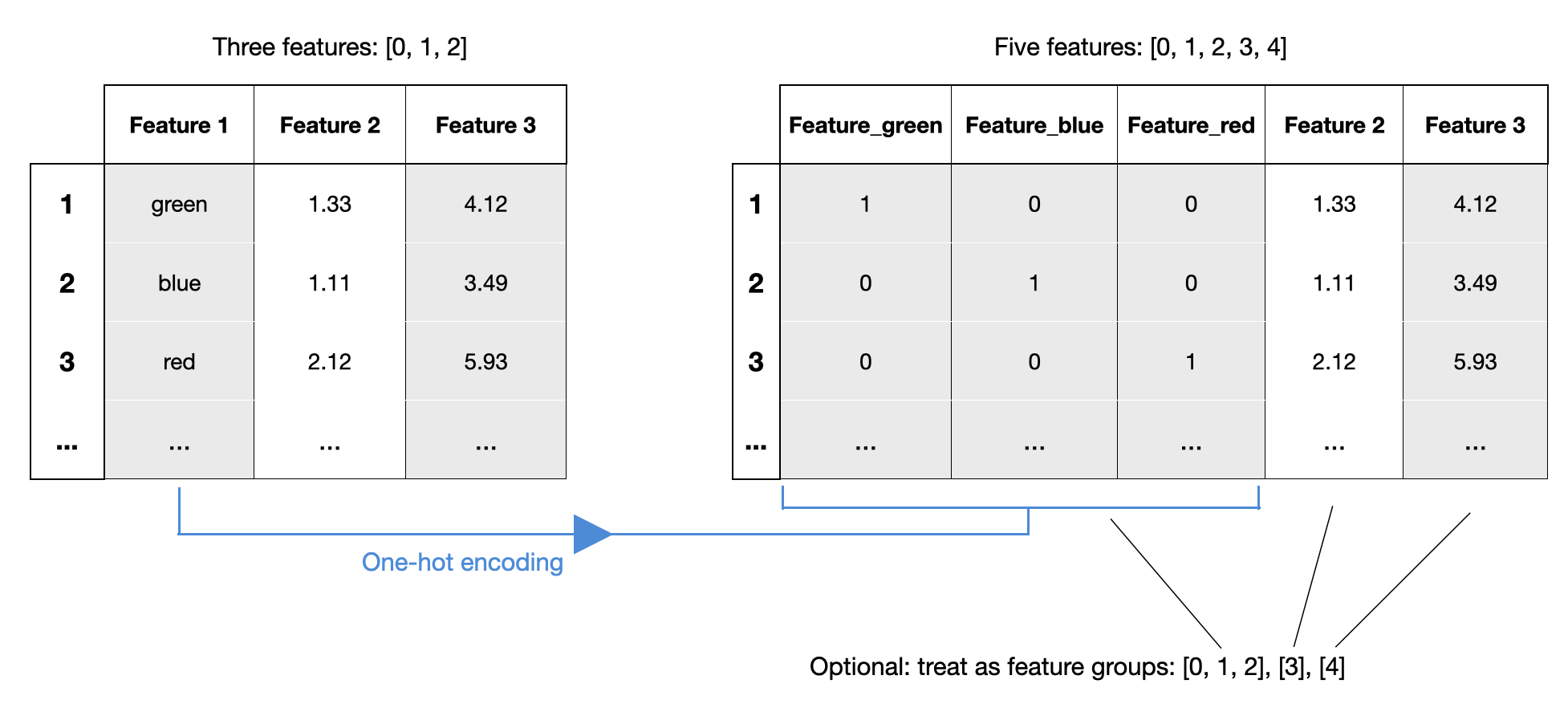
In the following example, we specify sepal length and sepal width as a feature group so that they are always selected together:

from sklearn.datasets import load_iris
import pandas as pd

iris = load_iris()
X = iris.data
y = iris.target

X_df = pd.DataFrame(X, columns=['sepal len', 'petal len',
                                'sepal wid', 'petal wid'])
X_df.head()

	sepal len	petal len	sepal wid	petal wid
0	5.1	3.5	1.4	0.2
1	4.9	3.0	1.4	0.2
2	4.7	3.2	1.3	0.2
3	4.6	3.1	1.5	0.2
4	5.0	3.6	1.4	0.2

from sklearn.neighbors import KNeighborsClassifier
from mlxtend.feature_selection import ExhaustiveFeatureSelector as EFS

knn = KNeighborsClassifier(n_neighbors=3)

efs1 = EFS(knn, 
           min_features=2,
           max_features=2,
           scoring='accuracy',
           feature_groups=[['sepal len', 'sepal wid'], ['petal len'], ['petal wid']],
           cv=3)

efs1 = efs1.fit(X_df, y)

print('Best accuracy score: %.2f' % efs1.best_score_)
print('Best subset (indices):', efs1.best_idx_)
print('Best subset (corresponding names):', efs1.best_feature_names_)

Features: 3/3

Best accuracy score: 0.97
Best subset (indices): (0, 2, 3)
Best subset (corresponding names): ('sepal len', 'sepal wid', 'petal wid')

Notice that the returned number of features is 3, since the number of min_features and max_features corresponds to the number of feature groups. I.e., we have 2 feature groups in ['sepal len', 'sepal wid'], ['petal wid'], but it expands to 3 features.

API

ExhaustiveFeatureSelector(estimator, min_features=1, max_features=1, print_progress=True, scoring='accuracy', cv=5, n_jobs=1, pre_dispatch='2n_jobs', clone_estimator=True, fixed_features=None, feature_groups=None)*

Exhaustive Feature Selection for Classification and Regression. (new in v0.4.3)

Parameters

estimator : scikit-learn classifier or regressor
min_features : int (default: 1)

Minumum number of features to select
max_features : int (default: 1)

Maximum number of features to select. If parameter feature_groups is not None, the number of features is equal to the number of feature groups, i.e. len(feature_groups). For example, if feature_groups = [[0], [1], [2, 3], [4]], then the max_features value cannot exceed 4.
print_progress : bool (default: True)

Prints progress as the number of epochs to stderr.
scoring : str, (default='accuracy')

Scoring metric in {accuracy, f1, precision, recall, roc_auc} for classifiers, {'mean_absolute_error', 'mean_squared_error', 'median_absolute_error', 'r2'} for regressors, or a callable object or function with signature scorer(estimator, X, y).
cv : int (default: 5)

Scikit-learn cross-validation generator or int. If estimator is a classifier (or y consists of integer class labels), stratified k-fold is performed, and regular k-fold cross-validation otherwise. No cross-validation if cv is None, False, or 0.
n_jobs : int (default: 1)

The number of CPUs to use for evaluating different feature subsets in parallel. -1 means 'all CPUs'.
pre_dispatch : int, or string (default: '2*n_jobs')

Controls the number of jobs that get dispatched during parallel execution if n_jobs > 1 or n_jobs=-1. Reducing this number can be useful to avoid an explosion of memory consumption when more jobs get dispatched than CPUs can process. This parameter can be: None, in which case all the jobs are immediately created and spawned. Use this for lightweight and fast-running jobs, to avoid delays due to on-demand spawning of the jobs An int, giving the exact number of total jobs that are spawned A string, giving an expression as a function of n_jobs, as in 2*n_jobs
clone_estimator : bool (default: True)

Clones estimator if True; works with the original estimator instance if False. Set to False if the estimator doesn't implement scikit-learn's set_params and get_params methods. In addition, it is required to set cv=0, and n_jobs=1.
fixed_features : tuple (default: None)

If not None, the feature indices provided as a tuple will be regarded as fixed by the feature selector. For example, if fixed_features=(1, 3, 7), the 2nd, 4th, and 8th feature are guaranteed to be present in the solution. Note that if fixed_features is not None, make sure that the number of features to be selected is greater than len(fixed_features). In other words, ensure that k_features > len(fixed_features).
feature_groups : list or None (default: None)

Optional argument for treating certain features as a group. This means, the features within a group are always selected together, never split. For example, feature_groups=[[1], [2], [3, 4, 5]] specifies 3 feature groups.In this case, possible feature selection results with k_features=2 are [[1], [2], [[1], [3, 4, 5]], or [[2], [3, 4, 5]]. Feature groups can be useful for interpretability, for example, if features 3, 4, 5 are one-hot encoded features. (For more details, please read the notes at the bottom of this docstring). New in mlxtend v. 0.21.0.

Attributes

best_idx_ : array-like, shape = [n_predictions]

Feature Indices of the selected feature subsets.
best_feature_names_ : array-like, shape = [n_predictions]

Feature names of the selected feature subsets. If pandas DataFrames are used in the fit method, the feature names correspond to the column names. Otherwise, the feature names are string representation of the feature array indices. New in v 0.13.0.
best_score_ : float

Cross validation average score of the selected subset.
subsets_ : dict

A dictionary of selected feature subsets during the exhaustive selection, where the dictionary keys are the lengths k of these feature subsets. The dictionary values are dictionaries themselves with the following keys: 'feature_idx' (tuple of indices of the feature subset) 'feature_names' (tuple of feature names of the feat. subset) 'cv_scores' (list individual cross-validation scores) 'avg_score' (average cross-validation score) Note that if pandas DataFrames are used in the fit method, the 'feature_names' correspond to the column names. Otherwise, the feature names are string representation of the feature array indices. The 'feature_names' is new in v. 0.13.0.

Notes

(1) If parameter feature_groups is not None, the number of features is equal to the number of feature groups, i.e. len(feature_groups). For example, if feature_groups = [[0], [1], [2, 3], [4]], then the max_features value cannot exceed 4.

(2) Although two or more individual features may be considered as one group
throughout the feature-selection process, it does not mean the individual
features of that group have the same impact on the outcome. For instance, in
linear regression, the coefficient of the feature 2 and 3 can be different
even if they are considered as one group in feature_groups.

(3) If both fixed_features and feature_groups are specified, ensure that each
feature group contains the fixed_features selection. E.g., for a 3-feature set
fixed_features=[0, 1] and feature_groups=[[0, 1], [2]] is valid;
fixed_features=[0, 1] and feature_groups=[[0], [1, 2]] is not valid.

Examples

For usage examples, please see http://rasbt.github.io/mlxtend/user_guide/feature_selection/ExhaustiveFeatureSelector/

Methods

fit(X, y, groups=None, fit_params)

Perform feature selection and learn model from training data.

Parameters

X : {array-like, sparse matrix}, shape = [n_samples, n_features]

Training vectors, where n_samples is the number of samples and n_features is the number of features. New in v 0.13.0: pandas DataFrames are now also accepted as argument for X.
y : array-like, shape = [n_samples]

Target values.
groups : array-like, with shape (n_samples,), optional

Group labels for the samples used while splitting the dataset into train/test set. Passed to the fit method of the cross-validator.
fit_params : dict of string -> object, optional

Parameters to pass to to the fit method of classifier.

Returns

self : object

fit_transform(X, y, groups=None, fit_params)

Fit to training data and return the best selected features from X.

Parameters

X : {array-like, sparse matrix}, shape = [n_samples, n_features]

Training vectors, where n_samples is the number of samples and n_features is the number of features. New in v 0.13.0: pandas DataFrames are now also accepted as argument for X.
y : array-like, shape = [n_samples]

Target values.
groups : array-like, with shape (n_samples,), optional

Group labels for the samples used while splitting the dataset into train/test set. Passed to the fit method of the cross-validator.
fit_params : dict of string -> object, optional

Parameters to pass to to the fit method of classifier.

Returns

Feature subset of X, shape={n_samples, k_features}

get_metric_dict(confidence_interval=0.95)

Return metric dictionary

Parameters

confidence_interval : float (default: 0.95)

A positive float between 0.0 and 1.0 to compute the confidence interval bounds of the CV score averages.

Returns

Dictionary with items where each dictionary value is a list with the number of iterations (number of feature subsets) as its length. The dictionary keys corresponding to these lists are as follows: 'feature_idx': tuple of the indices of the feature subset 'cv_scores': list with individual CV scores 'avg_score': of CV average scores 'std_dev': standard deviation of the CV score average 'std_err': standard error of the CV score average 'ci_bound': confidence interval bound of the CV score average

get_params(deep=True)

Get parameters for this estimator.

Parameters

deep : bool, default=True

If True, will return the parameters for this estimator and contained subobjects that are estimators.

Returns

params : dict

Parameter names mapped to their values.

set_params(params)

Set the parameters of this estimator.

The method works on simple estimators as well as on nested objects
(such as :class:`~sklearn.pipeline.Pipeline`). The latter have
parameters of the form ``<component>__<parameter>`` so that it's
possible to update each component of a nested object.

Parameters

**params : dict

Estimator parameters.

Returns

self : estimator instance

Estimator instance.

transform(X)

Return the best selected features from X.

Parameters

X : {array-like, sparse matrix}, shape = [n_samples, n_features]

Training vectors, where n_samples is the number of samples and n_features is the number of features. New in v 0.13.0: pandas DataFrames are now also accepted as argument for X.

Returns

Feature subset of X, shape={n_samples, k_features}

	Sepal length	Sepal width	Petal length	Petal width
0	5.1	3.5	1.4	0.2
1	4.9	3.0	1.4	0.2
2	4.7	3.2	1.3	0.2
3	4.6	3.1	1.5	0.2
4	5.0	3.6	1.4	0.2

	sepal len	petal len	sepal wid	petal wid
0	5.1	3.5	1.4	0.2
1	4.9	3.0	1.4	0.2
2	4.7	3.2	1.3	0.2
3	4.6	3.1	1.5	0.2
4	5.0	3.6	1.4	0.2

	Sepal length	Sepal width	Petal length	Petal width
0	5.1	3.5	1.4	0.2
1	4.9	3.0	1.4	0.2
2	4.7	3.2	1.3	0.2
3	4.6	3.1	1.5	0.2
4	5.0	3.6	1.4	0.2

	sepal len	petal len	sepal wid	petal wid
0	5.1	3.5	1.4	0.2
1	4.9	3.0	1.4	0.2
2	4.7	3.2	1.3	0.2
3	4.6	3.1	1.5	0.2
4	5.0	3.6	1.4	0.2

	Sepal length	Sepal width	Petal length	Petal width
0	5.1	3.5	1.4	0.2
1	4.9	3.0	1.4	0.2
2	4.7	3.2	1.3	0.2
3	4.6	3.1	1.5	0.2
4	5.0	3.6	1.4	0.2

	sepal len	petal len	sepal wid	petal wid
0	5.1	3.5	1.4	0.2
1	4.9	3.0	1.4	0.2
2	4.7	3.2	1.3	0.2
3	4.6	3.1	1.5	0.2
4	5.0	3.6	1.4	0.2