MultilayerPerceptron: A simple multilayer neural network

Implementation of a multilayer perceptron, a feedforward artificial neural network.

from mlxtend.classifier import MultiLayerPerceptron

Overview

Although the code is fully working and can be used for common classification tasks, this implementation is not geared towards efficiency but clarity – the original code was written for demonstration purposes.

Basic Architecture

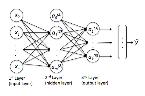
The neurons $x_0$ and $a_0$ represent the bias units ( $x_0=1$ , $a_0=1$ ).

The $i$ th superscript denotes the $i$ th layer, and the jth subscripts stands for the index of the respective unit. For example, $a_{1}^{(2)}$ refers to the first activation unit after the bias unit (i.e., 2nd activation unit) in the 2nd layer (here: the hidden layer)

$\begin{align} \mathbf{a^{(2)}} &= \begin{bmatrix} a_{0}^{(2)} \\ a_{1}^{(2)} \\ \vdots \\ a_{m}^{(2)} \end{bmatrix}. \end{align}$

Each layer $(l)$ in a multi-layer perceptron, a directed graph, is fully connected to the next layer $(l+1)$ . We write the weight coefficient that connects the $k$ th unit in the $l$ th layer to the $j$ th unit in layer $l+1$ as $w^{(l)}_{j, k}$ .

For example, the weight coefficient that connects the units

$a_0^{(2)} \rightarrow a_1^{(3)}$

would be written as $w_{1,0}^{(2)}$ .

Activation

In the current implementation, the activations of the hidden layer(s) are computed via the logistic (sigmoid) function $\phi(z) = \frac{1}{1 + e^{-z}}.$

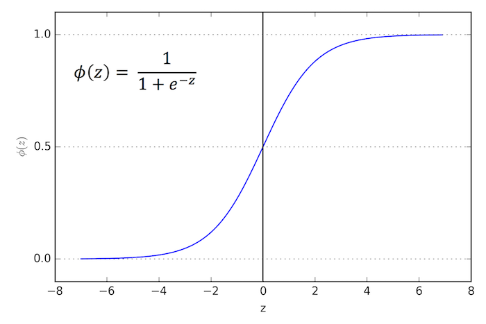
(For more details on the logistic function, please see classifier.LogisticRegression; a general overview of different activation function can be found here.)

Furthermore, the MLP uses the softmax function in the output layer, For more details on the logistic function, please see classifier.SoftmaxRegression.

References

D. R. G. H. R. Williams and G. Hinton. Learning representations by back-propagating errors. Nature, pages 323–533, 1986.
C. M. Bishop. Neural networks for pattern recognition. Oxford University Press, 1995.
T. Hastie, J. Friedman, and R. Tibshirani. The Elements of Statistical Learning, Volume 2. Springer, 2009.

Example 1 - Classifying Iris Flowers

Load 2 features from Iris (petal length and petal width) for visualization purposes:

from mlxtend.data import iris_data
X, y = iris_data()
X = X[:, [0, 3]]    

# standardize training data
X_std = (X - X.mean(axis=0)) / X.std(axis=0)

Train neural network for 3 output flower classes ('Setosa', 'Versicolor', 'Virginica'), regular gradient decent (minibatches=1), 30 hidden units, and no regularization.

Gradient Descent

Setting the minibatches to 1 will result in gradient descent training; please see Gradient Descent vs. Stochastic Gradient Descent for details.

from mlxtend.classifier import MultiLayerPerceptron as MLP

nn1 = MLP(hidden_layers=[50], 
          l2=0.00, 
          l1=0.0, 
          epochs=150, 
          eta=0.05, 
          momentum=0.1,
          decrease_const=0.0,
          minibatches=1, 
          random_seed=1,
          print_progress=3)

nn1 = nn1.fit(X_std, y)

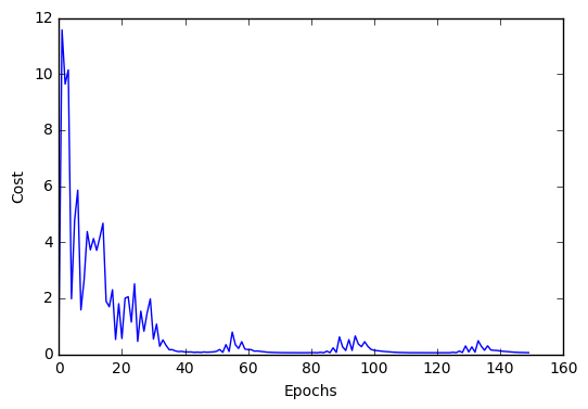
Iteration: 150/150 | Cost 0.06 | Elapsed: 0:00:00 | ETA: 0:00:00

from mlxtend.plotting import plot_decision_regions
import matplotlib.pyplot as plt

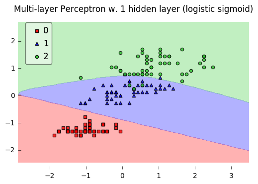
fig = plot_decision_regions(X=X_std, y=y, clf=nn1, legend=2)
plt.title('Multi-layer Perceptron w. 1 hidden layer (logistic sigmoid)')
plt.show()

png

import matplotlib.pyplot as plt
plt.plot(range(len(nn1.cost_)), nn1.cost_)
plt.ylabel('Cost')
plt.xlabel('Epochs')
plt.show()

png

print('Accuracy: %.2f%%' % (100 * nn1.score(X_std, y)))

Accuracy: 96.67%

Stochastic Gradient Descent

Setting minibatches to n_samples will result in stochastic gradient descent training; please see Gradient Descent vs. Stochastic Gradient Descent for details.

nn2 = MLP(hidden_layers=[50], 
          l2=0.00, 
          l1=0.0, 
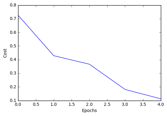
          epochs=5, 
          eta=0.005, 
          momentum=0.1,
          decrease_const=0.0,
          minibatches=len(y), 
          random_seed=1,
          print_progress=3)

nn2.fit(X_std, y)

plt.plot(range(len(nn2.cost_)), nn2.cost_)
plt.ylabel('Cost')
plt.xlabel('Epochs')
plt.show()

Iteration: 5/5 | Cost 0.11 | Elapsed: 00:00:00 | ETA: 00:00:00

png

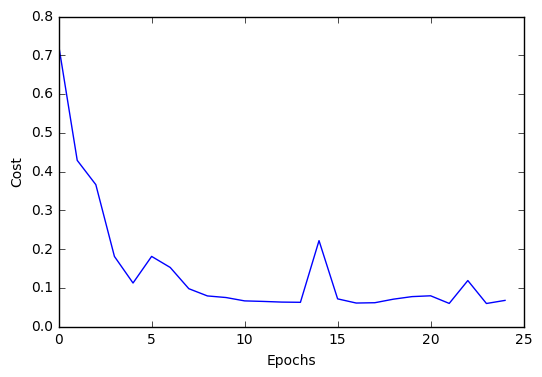
Continue the training for 25 epochs...

nn2.epochs = 25
nn2 = nn2.fit(X_std, y)

Iteration: 25/25 | Cost 0.07 | Elapsed: 0:00:00 | ETA: 0:00:00

plt.plot(range(len(nn2.cost_)), nn2.cost_)
plt.ylabel('Cost')
plt.xlabel('Epochs')
plt.show()

png

Example 2 - Classifying Handwritten Digits from a 10% MNIST Subset

Load a 5000-sample subset of the MNIST dataset (please see data.loadlocal_mnist if you want to download and read in the complete MNIST dataset).

from mlxtend.data import mnist_data
from mlxtend.preprocessing import shuffle_arrays_unison

X, y = mnist_data()
X, y = shuffle_arrays_unison((X, y), random_seed=1)
X_train, y_train = X[:500], y[:500]
X_test, y_test = X[500:], y[500:]

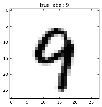
Visualize a sample from the MNIST dataset to check if it was loaded correctly:

import matplotlib.pyplot as plt

def plot_digit(X, y, idx):
    img = X[idx].reshape(28,28)
    plt.imshow(img, cmap='Greys',  interpolation='nearest')
    plt.title('true label: %d' % y[idx])
    plt.show()

plot_digit(X, y, 3500)

png

Standardize pixel values:

import numpy as np
from mlxtend.preprocessing import standardize

X_train_std, params = standardize(X_train, 
                                  columns=range(X_train.shape[1]), 
                                  return_params=True)

X_test_std = standardize(X_test,
                         columns=range(X_test.shape[1]),
                         params=params)

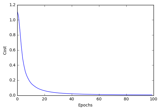
Initialize the neural network to recognize the 10 different digits (0-10) using 300 epochs and mini-batch learning.

nn1 = MLP(hidden_layers=[150], 
          l2=0.00, 
          l1=0.0, 
          epochs=100, 
          eta=0.005, 
          momentum=0.0,
          decrease_const=0.0,
          minibatches=100, 
          random_seed=1,
          print_progress=3)

Learn the features while printing the progress to get an idea about how long it may take.

import matplotlib.pyplot as plt

nn1.fit(X_train_std, y_train)

plt.plot(range(len(nn1.cost_)), nn1.cost_)
plt.ylabel('Cost')
plt.xlabel('Epochs')
plt.show()

Iteration: 100/100 | Cost 0.01 | Elapsed: 0:00:17 | ETA: 0:00:00

png

print('Train Accuracy: %.2f%%' % (100 * nn1.score(X_train_std, y_train)))
print('Test Accuracy: %.2f%%' % (100 * nn1.score(X_test_std, y_test)))

Train Accuracy: 100.00%
Test Accuracy: 84.62%

Please note that this neural network has been trained on only 10% of the MNIST data for technical demonstration purposes, hence, the lousy predictive performance.

API

MultiLayerPerceptron(eta=0.5, epochs=50, hidden_layers=[50], n_classes=None, momentum=0.0, l1=0.0, l2=0.0, dropout=1.0, decrease_const=0.0, minibatches=1, random_seed=None, print_progress=0)

Multi-layer perceptron classifier with logistic sigmoid activations

Parameters

eta : float (default: 0.5)

Learning rate (between 0.0 and 1.0)
epochs : int (default: 50)

Passes over the training dataset. Prior to each epoch, the dataset is shuffled if minibatches > 1 to prevent cycles in stochastic gradient descent.
hidden_layers : list (default: [50])

Number of units per hidden layer. By default 50 units in the first hidden layer. At the moment only 1 hidden layer is supported
n_classes : int (default: None)

A positive integer to declare the number of class labels if not all class labels are present in a partial training set. Gets the number of class labels automatically if None.
l1 : float (default: 0.0)

L1 regularization strength
l2 : float (default: 0.0)

L2 regularization strength
momentum : float (default: 0.0)

Momentum constant. Factor multiplied with the gradient of the previous epoch t-1 to improve learning speed w(t) := w(t) - (grad(t) + momentum * grad(t-1))
decrease_const : float (default: 0.0)

Decrease constant. Shrinks the learning rate after each epoch via eta / (1 + epoch*decrease_const)
minibatches : int (default: 1)

Divide the training data into k minibatches for accelerated stochastic gradient descent learning. Gradient Descent Learning if minibatches = 1 Stochastic Gradient Descent learning if minibatches = len(y) Minibatch learning if minibatches > 1
random_seed : int (default: None)

Set random state for shuffling and initializing the weights.
print_progress : int (default: 0)

Prints progress in fitting to stderr. 0: No output 1: Epochs elapsed and cost 2: 1 plus time elapsed 3: 2 plus estimated time until completion

Attributes

w_ : 2d-array, shape=[n_features, n_classes]

Weights after fitting.
b_ : 1D-array, shape=[n_classes]

Bias units after fitting.
cost_ : list

List of floats; the mean categorical cross entropy cost after each epoch.

Examples

For usage examples, please see https://rasbt.github.io/mlxtend/user_guide/classifier/MultiLayerPerceptron/

Methods

fit(X, y, init_params=True)

Learn model from training data.

Parameters

X : {array-like, sparse matrix}, shape = [n_samples, n_features]

Training vectors, where n_samples is the number of samples and n_features is the number of features.
y : array-like, shape = [n_samples]

Target values.
init_params : bool (default: True)

Re-initializes model parameters prior to fitting. Set False to continue training with weights from a previous model fitting.

Returns

self : object

predict(X)

Predict targets from X.

Parameters

X : {array-like, sparse matrix}, shape = [n_samples, n_features]

Training vectors, where n_samples is the number of samples and n_features is the number of features.

Returns

target_values : array-like, shape = [n_samples]

Predicted target values.

predict_proba(X)

Predict class probabilities of X from the net input.

Parameters

X : {array-like, sparse matrix}, shape = [n_samples, n_features]

Training vectors, where n_samples is the number of samples and n_features is the number of features.

Returns

Class probabilties : array-like, shape= [n_samples, n_classes]

score(X, y)

Compute the prediction accuracy

Parameters

X : {array-like, sparse matrix}, shape = [n_samples, n_features]

Training vectors, where n_samples is the number of samples and n_features is the number of features.
y : array-like, shape = [n_samples]

Target values (true class labels).

Returns

acc : float

The prediction accuracy as a float between 0.0 and 1.0 (perfect score).

ython

Keys	Action
`?`	Open this help
`n`	Next page
`p`	Previous page
`s`	Search