lift_score: Lift score for classification and association rule mining
Scoring function to compute the LIFT metric, the ratio of correctly predicted positive examples and the actual positive examples in the test dataset.
from mlxtend.evaluate import lift_score
Overview
In the context of classification, lift [1] compares model predictions to randomly generated predictions. Lift is often used in marketing research combined with gain and lift charts as a visual aid [2]. For example, assuming a 10% customer response as a baseline, a lift value of 3 would correspond to a 30% customer response when using the predictive model. Note that lift has the range .
There are many strategies to compute lift, and below, we will illustrate the computation of the lift score using a classic confusion matrix. For instance, let's assume the following prediction and target labels, where "1" is the positive class:
Then, our confusion matrix would look as follows:
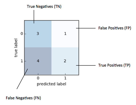
Based on the confusion matrix above, with "1" as positive label, we compute lift as follows:
Plugging in the actual values from the example above, we arrive at the following lift value:
An alternative way to computing lift is by using the support metric [3]:
Support is , where is the number of incidences of an observation and is the total number of samples in the datset. are the true positives, are true positives plus false negatives, and are true positives plus false positives. Plugging the values from our example into the equation above, we arrive at:
References
- [1] S. Brin, R. Motwani, J. D. Ullman, and S. Tsur. Dynamic itemset counting and implication rules for market basket data. In Proc. of the ACM SIGMOD Int'l Conf. on Management of Data (ACM SIGMOD '97), pages 265-276, 1997.
- [2] https://www3.nd.edu/~busiforc/Lift_chart.html
- [3] https://en.wikipedia.org/wiki/Association_rule_learning#Support
Example 1 - Computing Lift
This examples demonstrates the basic use of the lift_score function using the example from the Overview section.
import numpy as np
from mlxtend.evaluate import lift_score

y_target =    np.array([0, 0, 1, 0, 0, 1, 1, 1, 1, 1])
y_predicted = np.array([1, 0, 1, 0, 0, 0, 0, 1, 0, 0])

lift_score(y_target, y_predicted)
1.1111111111111112
Example 2 - Using lift_score in GridSearch
The lift_score function can also be used with scikit-learn objects, such as GridSearch:
from sklearn.datasets import load_iris
from sklearn.model_selection import train_test_split
from sklearn.model_selection import GridSearchCV
from sklearn.svm import SVC
from sklearn.metrics import make_scorer

# make custom scorer
lift_scorer = make_scorer(lift_score)


iris = load_iris()
X, y = iris.data, iris.target

X_train, X_test, y_train, y_test = train_test_split(
    X, y, test_size=0.2, stratify=y, random_state=123)

hyperparameters = [{'kernel': ['rbf'], 'gamma': [1e-3, 1e-4],
                     'C': [1, 10, 100, 1000]},
                   {'kernel': ['linear'], 'C': [1, 10, 100, 1000]}]

clf = GridSearchCV(SVC(), hyperparameters, cv=10,
                   scoring=lift_scorer)
clf.fit(X_train, y_train)

print(clf.best_score_)
print(clf.best_params_)
3.0
{'gamma': 0.001, 'kernel': 'rbf', 'C': 1000}
API
lift_score(y_target, y_predicted, binary=True, positive_label=1)
Lift measures the degree to which the predictions of a classification model are better than randomly-generated predictions.
The in terms of True Positives (TP), True Negatives (TN), False Positives (FP), and False Negatives (FN), the lift score is computed as: [ TP/(TP+FN) ] / [ (TP+FP) / (TP+TN+FP+FN) ]
Parameters
-
y_target: array-like, shape=[n_samples]True class labels.
-
y_predicted: array-like, shape=[n_samples]Predicted class labels.
-
binary: bool (default: True)Maps a multi-class problem onto a binary, where the positive class is 1 and all other classes are 0.
-
positive_label: int (default: 0)Class label of the positive class.
Returns
-
score: floatLift score in the range [0, ]
Examples
For usage examples, please see https://rasbt.github.io/mlxtend/user_guide/evaluate/lift_score/